Investment Growth Explained: Compounding With Clear Examples

Investment growth often looks mysterious at first: money goes in, time passes, and the balance becomes larger than what you deposited. The engine behind that change is usually compounding—the process where returns begin earning returns of their own.

This guide breaks down compounding from the ground up, then walks through practical examples (with numbers) you can apply to savings, retirement accounts, brokerage portfolios, and long-term goals. You’ll also learn how contribution timing, return rate, fees, taxes, and volatility can meaningfully change outcomes.

What “investment growth” really means

Your portfolio balance can rise from three main sources:

1. Contributions: money you add (one-time or recurring).
2. Investment returns: growth from price increases and earnings.
3. Reinvested earnings: dividends, interest, and distributions put back to work.

Compounding is mostly about the interaction between #2 and #3 over time. A return earned early can keep generating additional returns for decades.

Investment Compounding Growth: the core idea

If you invest a principal amount and it grows by a percentage each period, your next period’s growth is calculated on a larger base. That’s why compounding accelerates over time.

A simple way to describe it:

• In the early years, growth looks modest.
• Later, growth often dominates contributions, even if you keep depositing.

This is why time can matter as much as rate.

The basic compounding formula

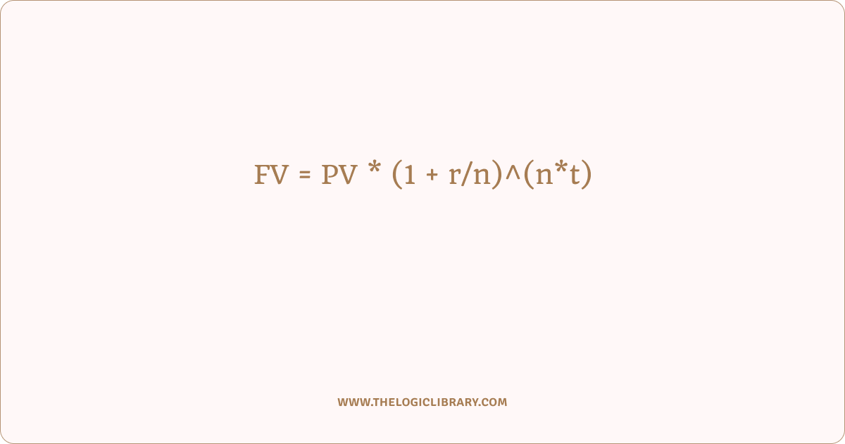
For a one-time investment (a lump sum), the future value with periodic compounding is:

FV = PV * (1 + r/n)^(n*t)

Where:

• FV = future value
• PV = present value (starting principal)
• r = annual return (as a decimal, e.g., 0.08 for 8%)
• n = number of compounding periods per year (e.g., 12 monthly)
• t = time in years

If compounding is annual (n = 1), it becomes:

FV = PV * (1 + r)^t

Continuous compounding

Some models use continuous compounding:

FV = PV * e^(r*t)

This is more theoretical for most personal investing, but it’s useful for comparisons.

Example 1: Lump sum compounding over time

Suppose you invest PV = 10,000 and earn r = 0.08 annually, compounded yearly for t = 20 years:

FV = 10000 * (1.08)^20

(1.08)^20 ≈ 4.660

So:

FV ≈ 10000 * 4.660 = 46,600

That’s a gain of 36,600 without adding another dollar after the first day. The large jump comes from time plus reinvested growth.

Now compare 10 years vs 20 years at the same return:

• FV10 = 10000 * (1.08)^10 ≈ 21,589
• FV20 = 46,600

The second decade adds about 25,011, more than the entire gain of the first decade. That’s compounding’s “late acceleration.”

Example 2: Monthly compounding vs annual compounding

Assume PV = 10,000, r = 0.08, t = 20.

Annual compounding:

FV_annual = 10000 * (1.08)^20 ≈ 46,600

Monthly compounding (n = 12):

FV_monthly = 10000 * (1 + 0.08/12)^(12*20)

(1 + 0.0066667)^(240) ≈ 4.926

So:

FV_monthly ≈ 10000 * 4.926 = 49,260

Same return rate, different compounding frequency: about 2,660 more over 20 years. In real markets, returns don’t arrive neatly by calendar, but this illustrates that more frequent reinvestment can slightly improve outcomes.

Investment Growth with recurring contributions

Most people invest repeatedly: monthly deposits to a retirement plan, weekly transfers to an index fund, or yearly additions from bonuses. This introduces a second growth driver: new money joining the compounding process.

Future value of a recurring contribution stream

If you contribute a fixed amount PMT each period and earn a periodic rate i, after N periods:

FV = PMT * (( (1 + i)^N - 1 ) / i)

Where:

• PMT = contribution each period
• i = periodic return rate
• N = total number of periods

If you invest monthly:

• i = r/12
• N = 12*t

If contributions happen at the beginning of each period (common with payroll deductions that hit early), multiply by (1 + i):

FV_begin = FV * (1 + i)

Example 3: $500 per month for 30 years

Assume:

• PMT = 500
• r = 0.08
• monthly contributions → i = 0.08/12
• t = 30
• N = 360

FV = 500 * ( ( (1 + 0.08/12)^360 - 1 ) / (0.08/12) )

(1 + 0.0066667)^360 ≈ 10.94

So:

FV ≈ 500 * ( (10.94 - 1) / 0.0066667 )
FV ≈ 500 * (9.94 / 0.0066667 )
FV ≈ 500 * 1,491
FV ≈ 745,500

Total contributions are 500 * 360 = 180,000. The rest—about 565,500—is growth.

This is why long horizons can make moderate contributions surprisingly powerful.

Example 4: Same contributions, different timelines

Keep PMT = 500 monthly, r = 0.08.

• 10 years (N = 120):
  (1.0066667)^120 ≈ 2.22
FV ≈ 500 * ( (2.22 - 1) / 0.0066667 )
FV ≈ 500 * 183
FV ≈ 91,500
• 20 years (N = 240):
  (1.0066667)^240 ≈ 4.93
FV ≈ 500 * ( (4.93 - 1) / 0.0066667 )
FV ≈ 500 * 589.5
FV ≈ 294,750
• 30 years (N = 360):
  FV ≈ 745,500

Notice the pattern: the final decade contributes an outsized portion of the ending balance. Contributions are steady, but compounded growth accelerates.

The “rule of 72” for quick intuition

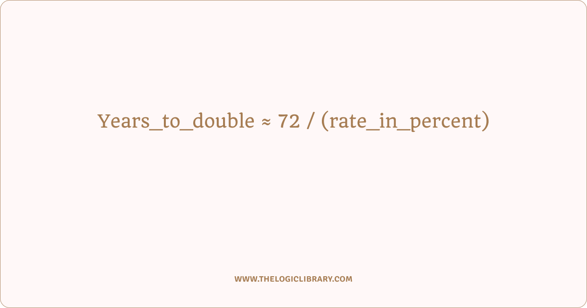
A quick estimate for doubling time is:

Years_to_double ≈ 72 / (rate_in_percent)

Examples:

• At 6%: 72/6 = 12 years to roughly double.
• At 9%: 72/9 = 8 years.
• At 3%: 72/3 = 24 years.

It’s an approximation, but it’s useful for sanity checks and comparisons.

Compounding with real-world messiness: volatility and sequence

Markets don’t deliver consistent returns each year. A portfolio might gain 25% one year and lose 15% the next. Over long periods, average returns can still be strong, but the order of returns can matter—especially when you are making withdrawals.

Geometric vs arithmetic average

If returns vary, the “simple average” isn’t the true compounding rate.

For annual returns r1, r2, ... rT, the compounded growth factor is:

Growth = Π(1 + rt)

The compounded annual growth rate (CAGR) is:

CAGR = ( (Ending / Beginning)^(1/T) ) - 1

A portfolio can have a high arithmetic average but a lower CAGR if volatility is high. This is one reason diversification can improve outcomes: not necessarily by boosting returns, but by smoothing the path.

Example 5: Same average, different result

Two-year scenario:

Path A: +50% then -50%
Start 100 → 150 → 75
Total return: -25%

Path B: +0% then +0%
Start 100 → 100 → 100
Total return: 0%

Arithmetic average of Path A is (50% + (-50%)) / 2 = 0%, yet you end down 25%. Compounding is multiplicative, not additive.

Contributions vs compounding: which matters more?

It’s tempting to obsess over return rates, but for many investors, the biggest controllable lever early on is contribution size and consistency. Return rate matters enormously over long horizons, but you can’t force markets to comply. You can control savings rate, fees, and diversification.

A useful mental model:

• Early stage: contributions drive most of your progress.
• Middle stage: contributions and growth both matter.
• Late stage: growth can dominate.

Fees: the quiet compounding killer

Fees reduce your effective return. A difference that looks small—like 1% per year—can translate into a large gap over decades.

If your gross return is r and annual fee is f, a simplified net return is:

r_net ≈ r - f

Then your future value becomes:

FV = PV * (1 + r_net)^t

Example 6: 8% return with 0.2% vs 1.2% annual fees

Assume:

• PV = 100,000
• t = 30
• Scenario 1: r_net = 0.08 - 0.002 = 0.078
• Scenario 2: r_net = 0.08 - 0.012 = 0.068

Compute:

FV1 = 100000 * (1.078)^30
(1.078)^30 ≈ 9.55
FV1 ≈ 955,000

FV2 = 100000 * (1.068)^30
(1.068)^30 ≈ 7.16
FV2 ≈ 716,000

Difference: about 239,000 on the same gross market return. Fees compound against you.

Investment Growth Taxes: compounding depends on the account type

Taxes can reduce compounding in two main ways:

1. Tax drag during the journey (taxable accounts): dividends and realized gains can create ongoing taxes, lowering reinvestment.
2. Tax at the end (tax-deferred accounts): growth compounds untaxed, but withdrawals may be taxed later.

A simplified model for taxable annual taxation on returns:

r_after_tax ≈ r * (1 - tax_rate)

Then apply:

FV = PV * (1 + r_after_tax)^t

Reality is more nuanced (different tax treatments for dividends, interest, short/long-term gains, and timing of realizations), but the concept is consistent: compounding is strongest when more of the return stays invested.

Inflation: the difference between “more money” and “more purchasing power”

A portfolio can grow in nominal terms while barely improving what it can buy. To convert a nominal return to an inflation-adjusted return, a common approximation is:

r_real ≈ (1 + r_nominal) / (1 + inflation) - 1

Example:

• r_nominal = 0.08
• inflation = 0.03

r_real ≈ 1.08/1.03 - 1 ≈ 0.0485 (about 4.85%)

Real returns are what build future lifestyle purchasing power.

Example 7: Growing wealth in today’s value

Assume PV = 100,000, r_nominal = 0.08, inflation = 0.03, t = 20.

Nominal future value:

FV_nominal = 100000 * (1.08)^20 ≈ 466,000

Real growth rate:

r_real ≈ 1.08/1.03 - 1 ≈ 0.0485

Inflation-adjusted future value (today’s purchasing power):

FV_real ≈ 100000 * (1.0485)^20

(1.0485)^20 ≈ 2.57
So:

FV_real ≈ 257,000

Both numbers are true; they answer different questions.

The power of starting earlier

Starting earlier does two things:

• gives your earliest contributions the longest runway,
• increases the portion of your timeline where growth has time to accelerate.

Example 8: Start at 25 vs 35 with the same monthly contribution

Assume:

• PMT = 500
• r = 0.08
• monthly
• Person A invests from age 25 to 65 → 40 years → N = 480
• Person B invests from age 35 to 65 → 30 years → N = 360

Person A:

FV_A = 500 * ( ( (1 + 0.08/12)^480 - 1 ) / (0.08/12) )

(1.0066667)^480 ≈ 24.6

FV_A ≈ 500 * ( (24.6 - 1) / 0.0066667 )
FV_A ≈ 500 * 3,540
FV_A ≈ 1,770,000

Person B (from earlier example): FV_B ≈ 745,500

Same monthly contribution, but the earlier start produces a dramatically larger result because the earliest dollars compound for an extra decade.

Contribution timing: end of month vs beginning of month

If you contribute at the beginning of each period instead of the end, every contribution gets one extra period of growth.

If FV_end is the end-of-period future value, then:

FV_begin = FV_end * (1 + i)

For monthly investing at r = 0.08, i = 0.0066667. Over long horizons, this can add up.

Compounding across different return rates

Small changes in return can create large differences over time. That’s not a promise of market performance—it’s a math lesson in sensitivity.

Example 9: Lump sum sensitivity

Assume PV = 50,000, t = 30.

• At 6%: FV = 50000 * (1.06)^30
(1.06)^30 ≈ 5.74 → FV ≈ 287,000
• At 8%: FV = 50000 * (1.08)^30
(1.08)^30 ≈ 10.06 → FV ≈ 503,000
• At 10%: FV = 50000 * (1.10)^30
(1.10)^30 ≈ 17.45 → FV ≈ 872,500

A 2% difference in assumed return can nearly double the ending balance over 30 years. That’s why fees, taxes, and risk exposure matter—because they influence effective long-term return.

What drives compounding in practice

Compounding isn’t just an equation. The real-world experience is shaped by behavior and structure.

1) Asset selection and diversification

Broad diversification can reduce the chance that one bad outcome derails the plan. It also helps investors stick with the strategy during downturns.

2) Reinvestment discipline

Returns only compound if they remain invested. Pulling earnings out interrupts the growth engine.

3) Consistent contributions

Regular investing makes compounding more robust because it keeps adding new money that can grow.

4) Staying invested through downturns

Volatility is normal. Long-term compounding typically requires enduring periods when results look disappointing.

5) Minimizing avoidable leakage

Fees, unnecessary trading costs, and tax inefficiency can all reduce the share of returns that remains in the portfolio to compound.

Building an “investment growth forecast” you can trust

A forecast shouldn’t be one magic number. It should be a range based on reasonable assumptions.

A simple approach:

1. Choose a time horizon t.
2. Pick three return assumptions:
   • conservative r_low
   • baseline r_mid
   • optimistic r_high
3. Estimate future value for each case using the same contribution plan.

For monthly contributions:

FV = PV*(1+i)^N + PMT * ( ( (1+i)^N - 1 ) / i )

Where:

• i = r/12
• N = 12*t

This includes both the starting balance and the recurring deposits.

Example 10: Forecast range

Assume:

• PV = 20,000
• PMT = 400 monthly
• t = 25 years → N = 300

Evaluate at 5%, 7%, 9%:

• r = 0.05 → i = 0.0041667
• r = 0.07 → i = 0.0058333
• r = 0.09 → i = 0.0075

You’ll often find the range between conservative and optimistic is very wide. That’s normal. The point of forecasting is planning resilience, not predicting.

Compounding during accumulation vs withdrawals

Compounding feels straightforward while you’re adding money. Withdrawals introduce a new risk: you might pull funds during a market decline, locking in losses and shrinking the base that could recover.

A simplified withdrawal model for a fixed withdrawal W each year from a portfolio earning r:

Balance_next = Balance_now*(1+r) - W

If W is too large relative to the portfolio and return sequence is unfavorable, the portfolio can deplete even if the “average return” seems adequate. That’s why withdrawal planning often uses conservative assumptions and buffers.

Common compounding misconceptions

“Compounding guarantees profits.”

No. Compounding describes how returns accumulate; it doesn’t guarantee returns are positive. Compounding works in reverse too: losses reduce the base.

“Averaging returns tells the whole story.”

Not when returns fluctuate. The order of returns affects outcomes, especially when withdrawing.

“I’ll wait until I have more money.”

Time is a major input. Starting smaller earlier can outperform starting bigger later.

“Fees don’t matter much.”

Over decades, fees compound against you and can become one of the largest controllable factors.

A practical compounding checklist

If you want compounding to work harder for you, focus on the levers you can control:

• Increase the contribution rate when income rises.
• Automate deposits so consistency is effortless.
• Keep a long horizon for long-term goals.
• Minimize avoidable fees and friction costs.
• Favor diversification that you can stick with.
• Reinvest earnings instead of consuming them.
• Build a plan for downturns so you don’t sell in panic.

Compounding is powerful, but it’s not fragile. It benefits from simple, repeatable habits.

FAQs

1) What is compounding in investing?

Compounding is the process where investment returns generate additional returns because growth is calculated on an ever-increasing balance. If a portfolio grows by r each period, the next period’s growth applies to the prior growth as well.

2) What is the difference between simple growth and compounded growth?

Simple growth applies returns only to the original principal. Compounded growth applies returns to principal plus previous returns. Lump-sum compounding is modeled by FV = PV*(1+r)^t.

3) How do monthly contributions compound?

Each contribution has its own time in the market. The combined effect is captured by FV = PMT * (((1+i)^N - 1)/i) where i is the periodic rate and N is the number of periods.

4) Does compounding happen if my investment pays dividends?

Yes—especially when dividends are reinvested. Reinvestment increases the number of shares (or units), which can increase future dividend payments and potential price appreciation.

5) How much does compounding frequency matter?

More frequent compounding can slightly increase the ending balance, all else equal. The difference between annual and monthly compounding is usually smaller than the impact of contribution size, fees, and time horizon.

6) What is CAGR and why is it useful?

CAGR is the constant annual rate that would produce the same start-to-end growth as the actual returns: CAGR = (Ending/Beginning)^(1/T) - 1. It summarizes uneven growth into one comparable figure.

7) Can compounding work against me?

Yes. Losses shrink the base, and future gains then compound from a lower level. A -50% loss requires a +100% gain to return to the starting point.

8) Why do fees matter so much over long periods?

Fees reduce the effective return that remains invested. Over time, the gap can be large because the fee savings also compounds. A simplified comparison uses r_net ≈ r - f in FV = PV*(1+r_net)^t.

9) How does inflation affect investment growth?

Inflation reduces purchasing power. To estimate inflation-adjusted growth, use r_real ≈ (1+r_nominal)/(1+inflation) - 1. This helps translate future balances into today’s value.

10) Is starting early more important than investing more?

Often, yes—because early contributions compound longer. A later start may require much larger deposits to catch up, depending on the time gap and return rate.

11) What is the rule of 72?

It estimates doubling time: Years_to_double ≈ 72 / rate%. It’s a quick approximation, not a precise calculator.

12) How do taxes change compounding?

Taxes can reduce reinvestment in taxable accounts (tax drag) or apply later in tax-deferred accounts. In simplified form, you can estimate r_after_tax ≈ r*(1-tax_rate) and compound with FV = PV*(1+r_after_tax)^t.

13) What is sequence risk?

Sequence risk is the impact of the order of returns—especially when withdrawing. Poor returns early in withdrawals can cause a portfolio to shrink faster, even if long-term averages look acceptable.

14) How can I model both a starting balance and monthly contributions together?

Use: FV = PV*(1+i)^N + PMT * (((1+i)^N - 1)/i) with i = r/12 and N = 12*t. This combines lump-sum growth and the contribution stream.

15) What’s the most reliable way to benefit from compounding?

Maintain a long horizon, contribute consistently, reinvest earnings, keep avoidable fees low, and choose a diversified approach you can hold through market declines.