Sampling Distribution: Definition, Formula & Example

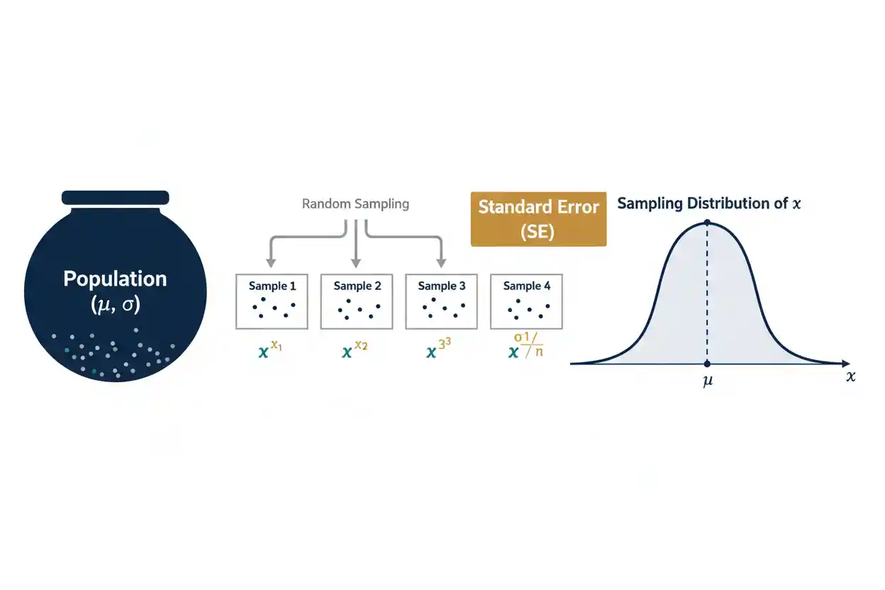
A sampling distribution is the probability distribution of a statistic across all possible samples of a specified size drawn under a defined sampling process. Instead of describing variation among individual observations, it describes how a statistic such as a sample mean, sample proportion, regression coefficient, variance, or other estimator would vary from sample to sample. This distinction is fundamental to statistical inference because an observed statistic is only one possible result from a sampling process. Its sampling distribution shows how much uncertainty is expected around that result and provides the foundation for standard errors, confidence intervals, hypothesis tests, critical values, and significance calculations. For example, individual observations in a population may have standard deviation σ, while sample means based on n independent observations have standard deviation σ/√n under the usual conditions.

That smaller spread explains why averages based on larger samples tend to be more stable. The shape of a sampling distribution depends on the statistic, population, sample size, and sampling design, so it should not be confused with either the raw-data distribution or the empirical distribution observed in one sample. Some sampling distributions are known exactly under specific assumptions, while others are approximated asymptotically or estimated through resampling. Understanding the sampling distribution therefore provides the bridge between descriptive sample calculations and probabilistic conclusions about unknown population quantities.

Sampling distributions are central to Statistics & Probability and especially to Inference & Regression. They explain why estimated quantities such as a Regression Slope and Regression Intercept have standard errors and why inferential thresholds can be constructed around those estimates.

What Is a Sampling Distribution?

Suppose a population has an unknown mean μ. A random sample of size n is drawn, and its sample mean is calculated:

x̄ = Σxᵢ / n

If another random sample of the same size is drawn from the same population, its sample mean will usually be different.

Repeated sampling would produce:

x̄₁, x̄₂, x̄₃, …

The probability distribution formed by those possible sample means is the sampling distribution of x̄.

The same principle applies to other statistics. Repeated samples could generate:

p̂₁, p̂₂, p̂₃, …

for sample proportions, or:

b₁,₁, b₁,₂, b₁,₃, …

for estimated regression slopes.

A sampling distribution therefore belongs to a statistic rather than directly to the individual observations.

Population Distribution vs Sample Distribution vs Sampling Distribution

These three ideas are easy to confuse.

A population distribution describes individual values in the population.

A sample distribution describes the observed individual values within one particular sample.

A sampling distribution describes the values of a statistic across repeated samples.

Suppose heights in a population have mean:

μ = 170 cm

and standard deviation:

σ = 10 cm

One sample of 25 individuals might contain heights ranging from 150 to 190 cm. That set of 25 observations has its own sample distribution.

If thousands of independent samples of size 25 were drawn and the mean of each sample calculated, those sample means would form a different distribution: the sampling distribution of x̄.

Its spread would typically be much smaller than the spread of individual heights.

Why Sampling Distributions Matter

Statistical inference asks questions about populations using limited samples.

Suppose a sample produces:

x̄ = 103

A single value does not tell us how uncertain that estimate is.

If sample means commonly vary by ±20 units from sample to sample, an observed mean of 103 may be highly imprecise.

If they usually vary by only ±0.5 units, 103 is a much more precise estimate.

The sampling distribution quantifies this variability.

Its standard deviation is called the standard error of the statistic.

That standard error is then used throughout inferential statistics to judge how far an observed estimate lies from a hypothesized value and how precisely a population parameter has been estimated.

Sampling Distribution of the Sample Mean

Let:

X₁, X₂, …, Xₙ

be independent observations from a population with mean μ and finite variance σ².

The sample mean is:

x̄ = (X₁ + X₂ + … + Xₙ) / n

Its expected value is:

E(x̄) = μ

This means the sample mean is an unbiased estimator of μ under the usual sampling conditions.

The variance of the sample mean is:

Var(x̄) = σ² / n

Therefore, its standard deviation is:

SD(x̄) = σ / √n

This standard deviation of the sampling distribution is the standard error when σ is known:

SE(x̄) = σ / √n

Worked Sampling Distribution Example

Suppose a population has:

μ = 100

σ = 20

and random samples of:

n = 25

are repeatedly drawn.

The expected value of the sample mean is:

E(x̄) = 100

The standard error is:

SE(x̄) = 20 / √25

SE(x̄) = 20 / 5

SE(x̄) = 4

Therefore, the sampling distribution of the sample mean is centered at 100 and has a standard deviation of 4.

Individual population observations vary with standard deviation 20, but sample means based on 25 observations vary with standard deviation only 4.

This illustrates the stabilizing effect of averaging.

Effect of Increasing Sample Size

The standard error of the mean is:

SE(x̄) = σ / √n

As n increases, the denominator increases and the sampling distribution becomes narrower.

Suppose:

σ = 20

For:

n = 25

we have:

SE = 20 / 5 = 4

For:

n = 100

we have:

SE = 20 / 10 = 2

For:

n = 400

we have:

SE = 20 / 20 = 1

Increasing the sample size from 25 to 100 reduces the standard error from 4 to 2.

Increasing it again from 100 to 400 reduces the standard error from 2 to 1.

Because n appears under a square root, quadrupling sample size approximately halves the standard error.

Why Larger Samples Are More Precise

A single observation can be far above or below the population mean. When many independent observations are averaged, positive and negative deviations tend to offset one another.

The variance calculation makes this precise.

If:

Var(Xᵢ) = σ²

and observations are independent, then:

Var(X₁ + … + Xₙ) = nσ²

Because the mean divides the total by n:

x̄ = (X₁ + … + Xₙ) / n

the variance becomes:

Var(x̄) = nσ² / n²

Var(x̄) = σ² / n

Taking the square root gives:

SD(x̄) = σ / √n

The increased precision of large-sample averages follows directly from this variance relationship.

Standard Error

The standard error is the standard deviation of a statistic’s sampling distribution.

For the sample mean when σ is known:

SE(x̄) = σ / √n

When σ is unknown, it is commonly estimated using:

Estimated SE(x̄) = s / √n

where s is the sample standard deviation.

Standard error should not be confused with standard deviation.

Standard deviation describes variation among individual observations.

Standard error describes sampling variation in an estimator or statistic.

Both measure spread, but they describe different distributions.

Standard Deviation vs Standard Error

Suppose individual observations have:

σ = 30

and:

n = 100

The population standard deviation remains:

30

because sample size does not alter how variable individual population observations are.

The sample mean’s standard error is:

30 / √100

= 3

Thus:

Standard deviation of observations = 30

Standard error of sample mean = 3

Reporting one in place of the other can substantially misrepresent uncertainty.

The standard error becomes smaller with sample size because it concerns the precision of an estimated statistic rather than individual variability.

The Central Limit Theorem and Sampling Distributions

One of the most important results in statistics concerns the shape of the sampling distribution of the mean.

Under suitable conditions, as sample size increases, the standardized sample mean approaches a standard normal distribution:

(x̄ − μ) / (σ / √n) → Normal(0,1)

in distribution.

Equivalently, for sufficiently large n under appropriate conditions:

x̄ ≈ Normal(μ, σ²/n)

even when the original population is not normally distributed.

This does not mean the population itself becomes normal.

It means the distribution of sample means becomes approximately normal.

The distinction is crucial.

Exact Normal Sampling Distribution

If the population itself is normally distributed:

X ∼ Normal(μ, σ²)

then the sample mean has an exact normal distribution for every sample size n under independent sampling:

x̄ ∼ Normal(μ, σ²/n)

No large-sample approximation is required.

For example, if:

X ∼ Normal(50, 12²)

and:

n = 9

then:

x̄ ∼ Normal(50, 12²/9)

The standard error is:

12 / 3 = 4

so:

x̄ ∼ Normal(50, 4²)

This exact result is stronger than an asymptotic central-limit approximation.

Non-Normal Population Example

Suppose individual observations are strongly right-skewed. One sample may contain many small values and a few very large ones.

For small n, the sampling distribution of x̄ may also remain visibly skewed.

As n grows, averaging increasingly stabilizes the statistic, and under appropriate finite-variance conditions the distribution of x̄ becomes more nearly normal.

However, the speed of convergence depends on the underlying population.

A mildly skewed population may require relatively few observations for a useful approximation.

A highly skewed or heavy-tailed population may require substantially more.

There is therefore no universal sample size at which every sampling distribution becomes adequately normal.

No Universal n = 30 Rule

A common shortcut says that:

n ≥ 30

guarantees an approximately normal sampling distribution of the mean.

This is not a universal theorem.

If the population is already approximately normal, a smaller sample may be sufficient.

If the population is extremely skewed, heavy-tailed, or contaminated by rare extreme values, a sample size of 30 may be inadequate.

The quality of the approximation depends on:

• population shape
• tail behavior
• existence of finite variance
• sample independence
• required accuracy

Sample size should therefore be interpreted in context rather than through a fixed cutoff.

Sampling Distribution of a Proportion

Suppose a binary outcome has population probability:

p

For a random sample of n independent Bernoulli observations, the sample proportion is:

p̂ = X / n

where X is the number of successes.

The expected value is:

E(p̂) = p

and its variance is:

Var(p̂) = p(1 − p) / n

Therefore:

SE(p̂) = √[p(1 − p) / n]

Under suitable sample-size conditions, the sampling distribution of p̂ can be approximated by a normal distribution.

The same general idea appears again: a sample statistic varies across repeated samples, and its standard error quantifies that variability.

Example: Sampling Distribution of a Proportion

Suppose:

p = 0.40

and:

n = 100

Then:

E(p̂) = 0.40

The standard error is:

SE(p̂) = √[(0.40)(0.60) / 100]

= √(0.24 / 100)

= √0.0024

≈ 0.049

Thus repeated sample proportions of size 100 would vary around 0.40 with a standard deviation of approximately 0.049 under the sampling model.

A sample proportion of 0.45 is therefore only about:

(0.45 − 0.40) / 0.049

≈ 1.02

standard errors above the population value.

Sampling Distribution of a Difference Between Means

Suppose two independent samples estimate population means μ₁ and μ₂.

The difference between sample means is:

x̄₁ − x̄₂

Its expected value is:

E(x̄₁ − x̄₂) = μ₁ − μ₂

If the samples are independent and population variances are σ₁² and σ₂²:

Var(x̄₁ − x̄₂) = σ₁²/n₁ + σ₂²/n₂

Therefore:

SE(x̄₁ − x̄₂) = √(σ₁²/n₁ + σ₂²/n₂)

This sampling distribution allows researchers to evaluate whether an observed difference between sample means is large relative to the variation expected from repeated sampling.

The same principle extends to many other estimators.

Sampling Distribution of a Regression Slope

The estimated Regression Slope b₁ varies from sample to sample.

Under the classical simple linear regression model:

Yᵢ = β₀ + β₁Xᵢ + εᵢ

each new random sample produces a new estimate:

b₁

The sampling distribution of b₁ is centered at β₁ under the standard unbiasedness conditions.

Its estimated standard error in the homoscedastic simple-regression framework is:

SE(b₁) = sₑ / √Sxx

where:

Sxx = Σ(xᵢ − x̄)²

The slope’s sampling distribution provides the basis for confidence intervals and tests of hypotheses such as:

H₀: β₁ = 0

An observed coefficient should therefore be interpreted as one realization from a distribution of possible estimates.

Sampling Distribution of a Regression Intercept

The Regression Intercept also varies across repeated samples.

In simple OLS regression, its estimated standard error has the form:

SE(b₀) = sₑ × √[1/n + x̄²/Sxx]

under the usual constant-variance assumptions.

The intercept may be estimated less precisely when the predictor’s zero point lies far from the center of the observed x-values.

This happens because small sampling changes in the slope can create larger differences in the extrapolated fitted value at zero.

The sampling distribution therefore quantifies uncertainty in the intercept just as it does for the slope.

Sampling Distribution and Residuals

Residuals and sampling distributions describe different types of variation.

A residual is:

eᵢ = yᵢ − ŷᵢ

It describes the prediction discrepancy for an observed case within one fitted sample.

A sampling distribution describes how a statistic such as:

x̄

p̂

b₁

or:

b₀

varies across repeated samples.

Residual variability contributes to uncertainty in regression coefficients, but a residual distribution should not be confused with the sampling distribution of a slope or intercept.

The two concepts operate at different levels.

Standardized Residuals vs Standardized Statistics

Standardized Residuals rescale individual residuals according to their expected residual variability.

A standardized test statistic instead usually rescales an estimator relative to its sampling distribution.

For example:

z = (x̄ − μ) / (σ / √n)

measures how far a sample mean lies from μ in sampling-distribution standard deviations.

Similarly:

t = (b₁ − β₁,0) / SE(b₁)

measures how far an estimated slope lies from its hypothesized value in estimated standard-error units.

Both involve standardization, but their targets differ.

A standardized residual evaluates an individual fitted observation; a standardized statistic evaluates an estimator relative to its sampling uncertainty.

Sampling Distribution and Significance Level

A Significance Level defines how much probability from the null sampling distribution is allocated to a rejection region.

Suppose a test statistic follows approximately:

Z ∼ Normal(0,1)

under H₀.

For a two-sided test with:

α = 0.05

the rejection regions commonly contain:

0.025

in each tail.

This produces approximate critical values:

−1.96 and +1.96

The significance threshold therefore has meaning only because the null sampling distribution tells us how probable different test-statistic values are when H₀ holds.

Without a reference sampling distribution, a test statistic such as 2.3 has no standalone inferential meaning.

Null Sampling Distribution

A null sampling distribution is the distribution of a statistic calculated under the conditions specified by H₀.

Suppose:

H₀: μ = 100

The sampling distribution of x̄ under the null is centered at:

100

If:

σ = 20

and:

n = 100

then:

SE(x̄) = 2

Under normal or appropriate approximate conditions:

x̄ ≈ Normal(100, 2²)

An observed sample mean of:

104

is therefore:

(104 − 100) / 2

= 2

standard errors above the null mean.

Hypothesis testing evaluates the observed statistic relative to this null distribution.

Test Statistics Are Based on Sampling Distributions

A standardized test statistic commonly follows the form:

Test statistic = (estimate − hypothesized parameter) / standard error

For a known-σ mean test:

z = (x̄ − μ₀) / (σ / √n)

For a t-based mean test:

t = (x̄ − μ₀) / (s / √n)

For a regression slope:

t = (b₁ − β₁,0) / SE(b₁)

Each test statistic compares an estimate’s observed deviation with the amount of deviation normally expected from sampling variation.

The sampling distribution turns a raw difference into an interpretable standardized quantity.

Sampling Distribution and Confidence Intervals

A confidence interval can often be understood as an estimate plus and minus a multiple of its standard error:

estimate ± critical value × standard error

For a known-σ population mean:

x̄ ± z* × σ/√n

This formula comes directly from the sampling distribution of x̄.

If:

x̄ ∼ Normal(μ, σ²/n)

then:

(x̄ − μ) / (σ/√n)

has a standard normal distribution.

Probability statements about that standardized sampling distribution can be rearranged algebraically to create an interval procedure for μ.

Confidence intervals are therefore inseparable from sampling distributions.

Sampling Distribution and P-Values

A p-value is also derived from a sampling distribution under H₀.

Suppose an observed statistic is:

z = 2.5

For a two-sided standard normal test, the p-value measures the probability of obtaining:

|Z| ≥ 2.5

under the null sampling distribution.

A small probability indicates that the observed statistic lies in a relatively unusual part of that distribution.

Thus standard errors, critical values, confidence intervals, p-values, and hypothesis tests are not separate statistical inventions. They are interconnected consequences of the behavior of statistics across repeated samples.

Sampling Variability

Sampling variability refers to the fact that different random samples produce different estimates.

Suppose a population mean is:

μ = 50

One sample may produce:

x̄ = 48.9

another:

x̄ = 51.2

and another:

x̄ = 50.3

None of these differences necessarily represents an error in data collection.

They are expected consequences of observing only part of the population.

The sampling distribution quantifies this natural sample-to-sample variability.

A statistic with a narrow sampling distribution is estimated more precisely than one with a wide sampling distribution.

Sampling Error

Sampling error is commonly defined as the difference between a sample statistic and the population parameter it estimates.

For a sample mean:

Sampling error = x̄ − μ

If:

μ = 50

and:

x̄ = 52

then:

sampling error = 2

This is not necessarily a mistake.

It is the random discrepancy produced by sampling variability.

The sampling distribution describes how sampling errors behave across repeated samples.

When the estimator is unbiased, its sampling distribution is centered on the population parameter, meaning positive and negative sampling errors balance in expectation.

Bias and Sampling Distribution

An estimator is unbiased for a parameter θ when:

E(θ̂) = θ

The sampling distribution is then centered at the true parameter.

If:

E(θ̂) ≠ θ

the estimator is biased.

Its bias is:

Bias(θ̂) = E(θ̂) − θ

An estimator can have low sampling variance but substantial bias.

Conversely, it can be unbiased but highly variable.

Therefore, a complete evaluation of an estimator considers both where its sampling distribution is centered and how widely it is spread.

Precision and bias are separate properties.

Precision

Precision refers to the concentration of an estimator’s sampling distribution.

A narrow distribution means repeated samples produce similar estimates.

A wide distribution means estimates fluctuate substantially from sample to sample.

Standard error provides a numerical measure of this spread.

Suppose two estimators are both unbiased:

Estimator A: SE = 1

Estimator B: SE = 10

Estimator A is much more precise.

However, precision alone does not guarantee accuracy if the estimator is systematically biased.

Bias vs Precision Example

Suppose the true parameter is:

θ = 100

Estimator A has a sampling distribution centered at:

100

with standard error:

10

Estimator B is centered at:

105

with standard error:

1

Estimator A is unbiased but relatively imprecise.

Estimator B is precise but biased upward by five units.

Neither property alone determines which estimator is preferable in every context.

This illustrates why the entire sampling distribution—its center and spread—is informative.

Mean Squared Error of an Estimator

A common measure combining variance and bias is mean squared error:

MSE(θ̂) = Var(θ̂) + [Bias(θ̂)]²

An unbiased estimator has:

Bias = 0

so:

MSE = Var(θ̂)

A slightly biased estimator can sometimes have lower MSE if its sampling variance is substantially reduced.

This illustrates a broader statistical principle: evaluating estimators requires more than asking whether their expected value equals the parameter.

The shape, variability, bias, and intended loss or decision criterion can all matter.

Sampling Without Replacement

The formula:

SE(x̄) = σ / √n

is commonly presented for independent sampling or effectively infinite populations.

When sampling without replacement from a finite population and the sample is a substantial fraction of that population, a finite population correction can be relevant:

FPC = √[(N − n) / (N − 1)]

Then:

SE(x̄) = (σ / √n) × √[(N − n)/(N − 1)]

where N is the population size.

If n is very small relative to N, the correction is close to 1.

If a large fraction of the population is observed, uncertainty falls because less of the population remains unobserved.

Example of Finite Population Correction

Suppose:

N = 1,000

n = 500

and:

σ = 20

Without the correction:

SE = 20 / √500

SE ≈ 0.894

The correction is:

√[(1,000 − 500) / (1,000 − 1)]

= √(500/999)

≈ 0.707

Therefore:

Corrected SE ≈ 0.894 × 0.707

≈ 0.632

Sampling half of a finite population without replacement provides more information than 500 independent draws from an effectively unlimited population.

Independence Matters

The familiar variance reduction:

Var(x̄) = σ²/n

depends on the dependence structure of the observations.

More generally:

Var(x̄) = 1/n² × Var(ΣXᵢ)

If observations are positively correlated, covariance terms increase the variance of the mean.

Therefore, 100 highly correlated observations do not necessarily provide the same precision as 100 independent observations.

Examples include repeated measurements, clustered students, family members, nearby geographic observations, and time-series data.

Ignoring dependence can produce a sampling distribution that is much narrower than the true one, leading to underestimated standard errors.

Effective Sample Size

When observations are dependent, the nominal row count n can overstate the amount of independent information.

A dataset may contain:

10,000 observations

but if those observations come from only a small number of highly correlated clusters, the effective information can be much smaller.

The exact effective sample size depends on the dependence structure and estimator.

This is why standard errors for clustered, repeated, or time-dependent data require methods designed for those sampling processes.

Sampling distributions are properties of both the statistic and the way the data are generated.

Sampling Design Matters

A sampling distribution is not determined solely by the values in a dataset.

It depends on the sampling procedure.

Simple random sampling, stratified sampling, cluster sampling, unequal-probability sampling, repeated measures, and convenience sampling have different inferential implications.

A formula derived under simple random sampling may be inappropriate for a complex survey.

Likewise, a standard regression standard error derived under independent observations may not represent a clustered experiment.

The sampling design must be reflected in the sampling distribution used for inference.

A Large Sample Does Not Remove Bias

Suppose a survey asks only visitors to one specialized website about national behavior.

Increasing the number of respondents from:

1,000

to:

1,000,000

can dramatically reduce sampling variability within that selected population.

It does not necessarily make the respondents representative of the national population.

The sampling distribution may become extremely narrow around a biased target.

Large samples improve precision under a sampling mechanism; they do not automatically correct selection bias, measurement bias, confounding, or model misspecification.

Resampling and Empirical Sampling Distributions

Sometimes an analytic sampling distribution is difficult to derive.

Resampling methods can approximate the behavior of a statistic computationally.

A common idea is to repeatedly construct resampled datasets, calculate the statistic for each one, and examine the resulting distribution.

The collection:

θ̂₁*, θ̂₂*, …, θ̂B*

can approximate aspects of the estimator’s sampling variability under the resampling framework.

Such methods are especially useful for statistics whose standard-error formulas are complicated.

However, resampling does not eliminate the need for a representative data-generating design. Repeatedly resampling biased observations generally reproduces the information structure present in those observations.

Sampling Distribution Is Theoretical, Not Necessarily Observed

In a real study, researchers normally observe only one actual sample.

They do not literally draw every possible sample from the population.

The sampling distribution is therefore often theoretical or conceptual.

Its properties may be derived mathematically from probability assumptions, approximated through asymptotic results, or estimated through resampling.

This does not make it imaginary in an unscientific sense. It represents the repeated-sampling behavior implied by the statistical model.

Inference depends on understanding that hypothetical repeated behavior even when only one realized sample is available.

Parameter vs Statistic

A parameter describes a population.

Examples include:

μ = population mean

p = population proportion

β₁ = population regression slope

A statistic is calculated from sample data.

Examples include:

x̄ = sample mean

p̂ = sample proportion

b₁ = estimated regression slope

Parameters are treated as fixed but unknown in standard frequentist inference.

Statistics vary from sample to sample.

Sampling distributions describe that variation in statistics.

This parameter-statistic distinction is one of the conceptual foundations of statistical inference.

Statistic vs Estimator vs Estimate

An estimator is a rule or formula used to estimate a population parameter.

For example:

x̄ = ΣXᵢ/n

is an estimator of μ.

Before data are observed, x̄ can be viewed as a random variable with a sampling distribution.

After a particular sample is observed, suppose:

x̄ = 52.3

The number 52.3 is the estimate obtained from that estimator.

The sampling distribution concerns the estimator across hypothetical repetitions rather than only the single numerical estimate observed.

Sampling Distribution and Degrees of Freedom

Some sampling distributions depend on degrees of freedom.

For example, when estimating a normal-population mean with unknown σ:

t = (x̄ − μ) / (s/√n)

follows Student’s t distribution under the classical assumptions with:

df = n − 1

In regression, coefficient t statistics commonly use residual degrees of freedom.

Chi-square and F distributions also use degrees-of-freedom parameters.

Degrees of freedom affect the shape of the sampling distribution and therefore change critical values, tail probabilities, and confidence intervals.

The correct reference distribution requires the correct degrees of freedom.

Why Student’s t Distribution Appears

If σ were known and the population mean estimator were normally distributed:

Z = (x̄ − μ) / (σ/√n)

would have a standard normal distribution.

When σ is unknown and replaced by s, the denominator itself varies from sample to sample.

Under normal-population conditions:

T = (x̄ − μ) / (s/√n)

follows Student’s t distribution.

The heavier tails of the t distribution reflect this additional uncertainty from estimating σ.

As degrees of freedom increase, s becomes a more stable estimate and the t distribution approaches the standard normal distribution.

Sampling Distribution of Variance

Sampling distributions are not restricted to means and proportions.

If observations come independently from a normal population, the sample variance has a chi-square relationship:

(n − 1)s² / σ² ∼ χ²(n − 1)

This result forms the basis for certain confidence intervals and hypothesis tests concerning population variance.

The sampling distribution is asymmetric because a variance cannot be negative.

This example demonstrates why not every statistic has an approximately bell-shaped sampling distribution, especially in small samples.

The shape depends on the statistic and the probability model.

Sampling Distribution of Ratios

Statistics based on ratios can have sampling distributions very different from those of simple means.

The F distribution, for example, arises from ratios of suitably scaled independent chi-square variables.

This makes it useful in variance comparisons and ANOVA-related inference.

Other ratios can have heavy-tailed or asymmetric distributions, especially when denominators can approach zero.

A statistic’s sampling distribution must therefore be derived or approximated for that statistic rather than assuming every estimator follows a normal distribution.

Normal Approximation Is Not Universal

The central limit theorem is powerful, but it does not imply that every statistic automatically becomes normally distributed for modest sample sizes.

Some estimators have:

• boundary constraints
• strong skewness
• heavy tails
• multimodality
• nonstandard behavior
• undefined moments under certain populations

In such cases, a normal approximation may be inaccurate or completely inappropriate.

The reference distribution should follow from the estimator and assumptions rather than from a general habit of using normal curves.

Sampling Distributions and Model Assumptions

Every analytical sampling distribution depends on assumptions.

These can include:

• independence
• identical distributions
• finite variance
• normality
• constant variance
• correct regression form
• known sampling probabilities
• suitable asymptotic conditions

If the assumptions fail, the theoretical sampling distribution may no longer describe the statistic correctly.

That can produce misleading standard errors, p-values, or confidence intervals.

Checking the model and data-generating process is therefore part of inference, not an optional step after calculating the statistic.

Sampling Distribution and Statistical Power

The width and location of a test statistic’s sampling distribution under alternative parameter values help determine statistical power.

Suppose H₀ is:

μ = 100

but the true mean is:

μ = 105

If sample size is small, the sampling distributions under 100 and 105 may overlap heavily.

It can then be difficult to distinguish the alternative from H₀.

As n increases, the standard error decreases and the distributions become narrower.

The same five-unit difference becomes easier to detect.

Thus increased power with larger sample size follows directly from the behavior of sampling distributions.

Common Sampling Distribution Mistakes

A common mistake is confusing the population distribution with the sampling distribution of a statistic. Individual observations may be highly variable while their sample mean has a much narrower distribution.

Another error is interpreting the sample’s histogram as the sampling distribution. One sample contains observations, not repeated realizations of the statistic.

A third mistake is treating standard deviation and standard error as equivalent. They describe different sources of variation.

Researchers also sometimes assume that increasing sample size fixes bias. It reduces random sampling variability but does not eliminate systematic selection or measurement problems.

Another misconception is that every sampling distribution is normal. Its shape depends on the statistic, population, sample size, and assumptions.

Finally, a sampling distribution cannot be interpreted independently of the sampling design that generated the statistic.

How to Find a Sampling Distribution

First identify the statistic of interest.

For example:

x̄

p̂

b₁

Then identify the sampling process and assumptions.

Next determine the statistic’s expected value:

E(statistic)

and its variance or standard error:

Var(statistic)

SE(statistic)

Then determine its distributional shape.

This may be exact, such as a normal, t, chi-square, or F distribution under specific assumptions, or approximate through an asymptotic theorem.

Finally, use that sampling distribution to answer the inferential question, such as calculating a confidence interval, tail probability, or significance threshold.

How to Interpret a Sampling Distribution

Suppose:

x̄ ≈ Normal(100, 2²)

This means repeated sample means generated under the specified sampling process are centered at 100 with standard deviation 2.

A sample mean of 104 lies:

(104 − 100) / 2

= 2

standard errors above the center.

A sample mean of 94 lies:

(94 − 100) / 2

= −3

standard errors below the center.

These standardized locations allow probabilities to be calculated from the sampling distribution.

The distribution therefore converts sample-to-sample variation into quantitative inferential statements.

Frequently Asked Questions

What is a sampling distribution?

A sampling distribution is the probability distribution of a statistic across repeated samples of a specified size drawn under a defined sampling process.

What is an example of a sampling distribution?

If many random samples of size n are drawn and the mean of each sample is calculated, the distribution of those sample means is the sampling distribution of x̄.

What is the sampling distribution of the mean?

Under independent sampling with population mean μ and variance σ²:

E(x̄) = μ

and:

Var(x̄) = σ²/n

so:

SE(x̄) = σ/√n

What is standard error?

Standard error is the standard deviation of a statistic’s sampling distribution.

What is the difference between standard deviation and standard error?

Standard deviation measures variation among observations. Standard error measures sampling variation in an estimated statistic.

Does the sampling distribution describe raw observations?

No. It describes possible values of a statistic across repeated samples.

Is a sample histogram a sampling distribution?

No. A sample histogram displays the observations within one sample. A sampling distribution requires repeated values of a statistic.

Is a sampling distribution always normal?

No. Some are normal exactly or approximately, while others can follow t, chi-square, F, skewed, or more complicated distributions.

What does the central limit theorem say about sample means?

Under suitable conditions, the standardized sample mean approaches a normal distribution as sample size increases.

Does the population have to be normal?

Not necessarily for a large-sample normal approximation of x̄, although the required sample size depends on population shape and tail behavior.

Does n = 30 guarantee normality?

No. There is no universal n = 30 rule.

What happens to the sampling distribution as n increases?

For many estimators such as the sample mean, the distribution becomes narrower because the standard error decreases.

Why does standard error decrease with n?

For the sample mean:

SE = σ/√n

so larger samples average out more random observation-level variability.

What is the sampling distribution of a sample proportion?

For independent Bernoulli sampling:

E(p̂) = p

and:

SE(p̂) = √[p(1 − p)/n]

Does a regression coefficient have a sampling distribution?

Yes. Repeated samples produce different estimated slopes and intercepts, allowing their uncertainty to be described by sampling distributions.

Are residuals a sampling distribution?

No. Residuals are observed-minus-predicted differences within a fitted sample. A sampling distribution describes a statistic across repeated samples.

What is sampling error?

Sampling error is the difference between a sample statistic and the population parameter it estimates.

Does larger sample size remove sampling error?

It generally reduces typical sampling error by narrowing the sampling distribution, but it does not guarantee an estimate exactly equals the population parameter.

Does larger sample size remove bias?

No. Large samples can estimate a biased target very precisely.

Why are sampling distributions important?

They provide the probability framework behind standard errors, confidence intervals, p-values, hypothesis tests, significance levels, and statistical power.

Key Takeaway

A sampling distribution describes how a statistic varies across repeated samples under a defined sampling process. For a sample mean based on independent observations with population mean μ and variance σ²:

E(x̄) = μ

Var(x̄) = σ²/n

and:

SE(x̄) = σ/√n

The sample mean is therefore centered on the population mean under the usual conditions, while its variability decreases as sample size grows. Similar sampling distributions exist for proportions, regression coefficients, variances, differences, and many other statistics.

The concept is distinct from both the population distribution and the observed distribution inside a single sample. Individual data describe units; a sampling distribution describes an estimator or statistic. Its spread determines standard error, its shape determines reference probabilities, and its location relative to a null value supports statistical testing.

Most importantly, sampling distributions explain why sample estimates are uncertain and how that uncertainty can be quantified. Their validity depends on the statistic, sampling design, dependence structure, population behavior, and model assumptions. Once those conditions are understood, the sampling distribution becomes the central probability mechanism connecting observed samples with inference about unknown population quantities.