Significance Level: Definition, Formula & Example

The significance level is a probability threshold used in statistical hypothesis testing to control how readily a testing procedure rejects a null hypothesis. It is conventionally represented by the Greek letter α and is commonly set before examining the test result. In a correctly calibrated test with a simple null hypothesis, α represents the probability of rejecting the null hypothesis when that null hypothesis is actually true, which is the probability of a Type I error. A significance level of 0.05 therefore means that the testing rule is designed to falsely reject a true null hypothesis about 5% of the time across repeated applications under the null model and required assumptions.

It does not mean there is a 5% probability that the null hypothesis is true, nor does it mean a statistically significant result has a 95% probability of being correct. The significance level determines the rejection region of the relevant reference distribution and provides the threshold against which a p-value can be compared. Smaller α values require stronger evidence before rejection and reduce the probability of Type I error, but they generally also reduce statistical power when other conditions remain unchanged. The appropriate significance level therefore reflects an error-control decision rather than a universal scientific constant.

The significance level is a core concept within Statistics & Probability and Inference & Regression. Its meaning depends on the relevant Sampling Distribution, because α defines how much probability from the null reference distribution is assigned to the rejection region.

What Is a Significance Level?

The significance level is written:

α

and represents the probability threshold chosen for a hypothesis-testing procedure.

For a simple null hypothesis:

α = P(reject H₀ | H₀ is true)

Suppose:

α = 0.05

The testing rule is calibrated so that, when H₀ is true and the model assumptions hold, the probability of falling into the rejection region is 0.05.

This is a long-run repeated-sampling statement.

It does not mean that after one particular test rejects H₀, there is a 5% probability that the rejection is wrong.

The significance level describes the operating behavior of the procedure under H₀ rather than assigning a probability to the truth of a hypothesis after data have been observed.

Significance Level Formula

The fundamental relationship is:

α = P(Type I error)

For a simple null hypothesis:

α = P(reject H₀ | H₀ true)

If a test uses:

α = 0.01

the procedure permits a 1% probability of rejecting H₀ when H₀ is true under the specified model.

If:

α = 0.10

the corresponding Type I error probability is 10%.

Common significance levels include:

α = 0.10

α = 0.05

α = 0.01

The choice depends on the consequences of false rejection, the research context, established conventions, and the broader decision framework.

Significance Level and Type I Error

A Type I error occurs when:

H₀ is true

but the test concludes:

Reject H₀

Suppose a quality-control system tests:

H₀: production process is operating at the specified population mean

If the process truly satisfies the null condition but the statistical test rejects it, a Type I error has occurred.

At:

α = 0.05

the procedure is designed so that this false rejection happens with probability 0.05 under H₀, assuming the statistical model and testing procedure are correctly specified.

A lower significance level makes false rejection less frequent, but it also makes the test more conservative.

Worked Example

Suppose a researcher tests:

H₀: μ = 100

against:

H₁: μ ≠ 100

and chooses:

α = 0.05

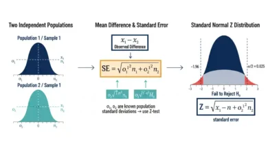
Assume the resulting standardized statistic follows a standard normal distribution under H₀:

Z ∼ Normal(0,1)

Because the test is two-sided, the total significance level is divided between the two tails:

α/2 = 0.05/2

α/2 = 0.025

The standard normal values leaving 2.5% in each tail are approximately:

−1.96 and +1.96

Therefore, the rejection rule is:

Reject H₀ if z < −1.96 or z > 1.96

Equivalently:

Reject H₀ if |z| > 1.96

The central 95% of the null distribution forms the non-rejection region, while the outer 5% forms the rejection region.

Example With an Observed Test Statistic

Suppose the test produces:

z = 2.30

The significance level remains:

α = 0.05

and the upper critical boundary is:

1.96

Because:

2.30 > 1.96

the statistic falls inside the rejection region.

The decision is:

Reject H₀

The same conclusion can be reached using the p-value. A two-sided z statistic of 2.30 has a p-value of approximately:

p ≈ 0.021

Since:

0.021 < 0.05

the test rejects H₀.

The significance level and critical-value approaches therefore express the same decision rule from different perspectives.

P-Value vs Significance Level

The p-value and significance level serve different roles.

The significance level:

α

is the threshold chosen for the testing procedure.

The p-value:

p

is calculated from the observed data and measures how extreme the test statistic is under H₀ according to the test definition.

The standard decision rule is:

If p ≤ α, reject H₀.

If p > α, fail to reject H₀.

Suppose:

p = 0.032

At:

α = 0.05

we have:

0.032 < 0.05

so H₀ is rejected.

At:

α = 0.01

we have:

0.032 > 0.01

so H₀ is not rejected at the 1% significance level.

The observed p-value has not changed. Only the required evidence threshold has changed.

Significance Level Should Usually Be Chosen Before the Result

The significance level should generally be defined before looking at the observed p-value or test statistic.

Suppose a researcher initially intends to use:

α = 0.05

but obtains:

p = 0.07

Changing the threshold afterward to:

α = 0.10

simply to obtain a statistically significant result makes the testing decision data-dependent.

The stated Type I error interpretation no longer cleanly describes a procedure that was fixed in advance.

A defensible analysis determines the testing rule according to the research design, consequences of errors, or established methodological standards rather than adjusting α to obtain a preferred conclusion.

Why 0.05 Is Common

The value:

α = 0.05

is widely used because it became a conventional compromise between requiring strong evidence and retaining useful ability to detect genuine effects.

It is not a mathematical law.

There is nothing inherently true or false about a result solely because its p-value falls just above or below 0.05.

For example:

p = 0.049

and:

p = 0.051

represent almost identical levels of incompatibility with the null model.

Yet a strict α = 0.05 decision rule places them on opposite sides of the rejection threshold.

This illustrates why statistical results should not be reduced to a significant/not-significant label without considering magnitude and uncertainty.

Choosing a Smaller Significance Level

Suppose the consequences of falsely rejecting H₀ are severe.

A researcher might choose:

α = 0.01

instead of:

α = 0.05

This makes the rejection region smaller and requires a more extreme test result before H₀ is rejected.

For a two-sided standard normal test:

At:

α = 0.05

the critical values are approximately:

±1.96

At:

α = 0.01

they are approximately:

±2.576

A statistic such as:

z = 2.20

would reject H₀ at the 5% level but not at the 1% level.

A smaller α therefore imposes stronger evidence requirements.

Choosing a Larger Significance Level

A larger α makes rejection easier.

For a two-sided standard normal test:

α = 0.10

corresponds to approximate critical values:

±1.645

The rejection region now contains 10% of the null distribution rather than 5%.

This increases sensitivity to departures from H₀ but also increases the probability of falsely rejecting H₀ when it is true.

A larger significance level can be reasonable in contexts where missing a genuine effect is especially costly relative to a false positive, but the tradeoff should be intentional rather than chosen merely to produce significance.

One-Tailed Significance Level

Suppose the hypotheses are:

H₀: μ = μ₀

H₁: μ > μ₀

For a right-tailed test with:

α = 0.05

the entire 5% rejection probability is placed in the upper tail.

For a standard normal statistic, the critical value is approximately:

zcritical = 1.645

The rejection rule is:

Reject H₀ if z > 1.645

This differs from the two-sided α = 0.05 critical value:

1.96

because a two-sided test divides the total α between two tails.

Left-Tailed Significance Level

For:

H₀: μ = μ₀

H₁: μ < μ₀

the rejection region lies entirely in the lower tail.

With:

α = 0.05

the standard normal critical value is approximately:

zcritical = −1.645

The decision rule becomes:

Reject H₀ if z < −1.645

A sufficiently large positive statistic would not reject H₀ in this left-tailed procedure because it points in the opposite direction from the specified alternative.

The direction of the test should therefore be determined by the research question before seeing the data.

Two-Tailed Significance Level

A two-sided test evaluates deviations in either direction:

H₀: parameter = null value

H₁: parameter ≠ null value

With:

α = 0.05

and a symmetric reference distribution:

α/2 = 0.025

is placed in each tail.

For a standard normal statistic:

zcritical ≈ ±1.96

For a t statistic, the corresponding critical values depend on the degrees of freedom.

The total rejection probability remains α even though it is divided across two regions.

Significance Level and Critical Values

A critical value is the boundary separating the rejection region from the non-rejection region.

The significance level determines where that boundary must be placed in the null distribution.

For example, in an upper-tailed standard normal test:

P(Z > zcritical) = α

If:

α = 0.05

then:

zcritical ≈ 1.645

If:

α = 0.01

then:

zcritical ≈ 2.326

As α decreases, the critical value moves farther into the tail.

This is why smaller significance levels require more extreme test statistics.

Significance Level Depends on the Reference Distribution

The same α does not imply the same numerical critical value for every statistical test.

At:

α = 0.05

a standard normal test can use:

±1.96

for a two-sided procedure.

A t-test uses critical values from Student’s t distribution, which depend on degrees of freedom.

An ANOVA uses an upper-tail F critical value.

A chi-square test uses a chi-square reference distribution.

The significance level tells us how much probability belongs in the rejection region. The relevant Sampling Distribution determines the numerical cutoff that creates that probability.

Significance Level and Confidence Level

For many standard two-sided procedures, a significance level α corresponds to a confidence level:

Confidence level = 1 − α

Thus:

α = 0.05

corresponds to:

1 − 0.05 = 0.95

or a 95% confidence level.

Similarly:

α = 0.01

corresponds to:

99% confidence

for the matching interval procedure.

If a compatible 95% confidence interval excludes the null value, the corresponding two-sided α = 0.05 test generally rejects that null value.

This relationship applies when the test and confidence interval are constructed from compatible inferential procedures.

Example With a Confidence Interval

Suppose a mean difference has a 95% confidence interval:

2.1 to 7.3

and the null hypothesis is:

H₀: difference = 0

Because:

0

lies outside the interval, the corresponding compatible two-sided test rejects H₀ at:

α = 0.05

If the interval were:

−1.2 to 6.0

zero would lie inside the interval, corresponding to failure to reject the zero-difference null using the matching 5% two-sided procedure.

The interval provides additional information because it shows the range of parameter values compatible with the data rather than only whether one benchmark crosses a significance threshold.

Significance Level and Statistical Power

Statistical Power is the probability of rejecting H₀ when a specified alternative is true.

If:

β = probability of Type II error

then:

Power = 1 − β

Holding sample size, effect size, variance, and test structure constant, reducing α generally reduces power.

Why?

A smaller α pushes the rejection boundary farther into the tail, so a more extreme result is required to reject H₀.

This decreases false positives but also makes genuine alternatives harder to detect.

The choice of significance level therefore participates in a tradeoff between Type I error control and statistical power.

Example of the Alpha-Power Tradeoff

Suppose a test initially uses:

α = 0.05

and rejects H₀ when:

z > 1.645

in a right-tailed standard normal procedure.

Now reduce the significance level to:

α = 0.01

The rejection boundary becomes:

z > 2.326

A true effect that often produces z statistics between 1.7 and 2.2 would frequently be detected under the first rule but missed under the second.

The lower α reduces false rejection under H₀ but also lowers the probability of detection under that alternative.

This tradeoff can often be counteracted by increasing the amount of independent information, such as through a larger sample.

Sample Size Does Not Change Alpha

Once α has been chosen, increasing sample size does not itself change the significance level.

If:

α = 0.05

the Type I error threshold remains 5% under a correctly calibrated procedure regardless of whether:

n = 20

or:

n = 20,000

What sample size changes is the precision of the estimator and therefore the power of the test against non-null alternatives.

Larger samples usually produce smaller standard errors, making modest departures from H₀ easier to detect.

This is why very large studies can produce statistical significance for effects that are numerically tiny.

Significance Level vs Statistical Significance

A significance level is the threshold:

α

Statistical significance is the decision obtained when the observed result crosses that threshold.

If:

p = 0.03

and:

α = 0.05

the result is statistically significant at the 5% level.

If:

α = 0.01

the same p-value is not statistically significant at the 1% level.

Therefore, a result should ideally be described in terms of its actual p-value and effect estimate rather than being labeled significant without specifying the threshold used.

Statistical Significance vs Practical Importance

Suppose an enormous study estimates a mean difference of:

0.02 units

with:

p < 0.001

The result crosses even a stringent significance level.

But a difference of 0.02 units may be practically meaningless.

Now consider a small study estimating:

10 units

with:

p = 0.08

The observed effect is much larger but less precisely estimated.

The significance level controls an inferential error rate; it does not define the minimum effect that matters in the real world.

Practical importance should be evaluated using effect magnitude, confidence intervals, costs, benefits, and domain-specific thresholds.

Type II Error

A Type II error occurs when the test fails to reject H₀ even though the relevant alternative is true.

Its probability is:

β

Unlike α, β usually depends on the particular alternative effect size.

For example, a test can have low probability of detecting a tiny effect but very high probability of detecting a large effect.

The relationship:

Power = 1 − β

makes clear that controlling α alone does not describe the complete performance of a hypothesis test.

A good study design considers both false-positive control and the ability to detect effects that are substantively important.

Alpha Is Not the False Discovery Rate

Suppose:

α = 0.05

This does not mean that 5% of statistically significant findings are false.

Alpha means:

P(reject H₀ | H₀ true) = 0.05

under the relevant procedure.

The probability that H₀ is true among rejected hypotheses depends on additional information, including how frequently null hypotheses are actually true, test power, selection procedures, and the number of analyses performed.

Therefore:

Type I error rate ≠ proportion of significant results that are false

This distinction is important when interpreting large collections of hypothesis tests.

Significance Level in Regression

Suppose a simple regression estimates a Regression Slope b₁ and tests:

H₀: β₁ = 0

A conventional t statistic may be:

t = b₁ / SE(b₁)

The selected significance level determines the rejection boundary from the relevant t distribution.

For example:

α = 0.05

might require:

|t| > tcritical

for a two-sided slope test.

If the statistic crosses that boundary, the data provide evidence that the population linear slope differs from zero under the model assumptions.

The significance level does not determine how large the slope is or whether it is practically meaningful.

Significance Level and Regression Assumptions

The intended Type I error interpretation assumes the statistical test is calibrated correctly.

If regression assumptions are badly violated, the nominal significance level may not equal the actual false-positive probability.

For example, strongly dependent observations treated as independent can produce standard errors that are too small.

This can make a nominal:

α = 0.05

test reject much more frequently than 5% under an appropriate null process.

Likewise, severe variance misspecification or inappropriate distributional assumptions can distort inference.

The number printed as α is therefore only meaningful when the testing procedure and assumptions support its calibration.

Residuals and Significance Testing

Residuals help assess whether a regression model is behaving consistently with assumptions used for inference.

Patterns such as:

strong curvature

changing residual spread

temporal dependence

or:

extreme influential observations

can signal problems with the model or standard-error calculation.

These issues matter because significance tests depend on correctly representing sampling uncertainty.

A p-value below α should not be interpreted mechanically while ignoring strong evidence that the underlying test is misspecified.

Standardized Residuals Are Not Significance Levels

Standardized Residuals express an individual residual relative to an estimate of its expected residual variability.

Analysts sometimes use heuristic values such as:

±2

or:

±3

to flag observations for closer examination.

These diagnostic cutoffs are not the same thing as choosing:

α = 0.05

for a hypothesis test.

A standardized residual threshold concerns unusual observations within a fitted model, while the significance level controls the rejection probability of a formal test under H₀.

Both use ideas about reference distributions, but they answer different statistical questions.

Significance Level and Multiple Testing

Suppose 20 independent hypotheses are all truly null and each is tested at:

α = 0.05

Each individual test has a 5% Type I error probability.

However, the probability of observing at least one false rejection across the collection can be much larger than 5%.

Under independence:

P(no false rejections) = (1 − 0.05)²⁰

≈ 0.358

Therefore:

P(at least one false rejection) ≈ 1 − 0.358

≈ 0.642

or about 64.2%.

This illustrates why a per-test significance level and a family-level error probability are not the same quantity.

Bonferroni Example

One simple way to control the familywise error rate across m planned tests is the Bonferroni threshold:

αindividual = αfamily / m

Suppose:

αfamily = 0.05

and:

m = 10

Then:

αindividual = 0.05 / 10

αindividual = 0.005

Each individual hypothesis would need:

p ≤ 0.005

to meet this particular familywise criterion.

Bonferroni control can be conservative, especially when tests are numerous or correlated, and other multiplicity procedures exist.

The broader lesson is that the appropriate significance threshold depends partly on the family of inferences being made.

Repeated Testing Can Change the Actual Error Rate

Suppose a researcher plans a fixed-sample test at:

α = 0.05

but repeatedly checks the result after every few new observations and stops immediately when significance appears.

A conventional fixed-sample significance threshold may no longer provide its intended 5% Type I error rate under this unplanned repeated testing.

Likewise, repeatedly trying models, outcomes, subgroups, or exclusion rules until one produces:

p < 0.05

changes the overall probability of a false-positive finding.

The significance level belongs to the full testing procedure, not merely to the final comparison shown in a report.

Significance Level and One-Sided Testing

A one-sided test can provide more power in one prespecified direction because all of α is allocated to one tail.

For example, with:

α = 0.05

a right-tailed z-test has:

zcritical ≈ 1.645

while a two-sided test has:

zcritical ≈ 1.96

in its upper tail.

However, the one-sided test provides no rejection region for an effect in the opposite direction.

If a treatment could plausibly cause either meaningful benefit or meaningful harm, a two-sided procedure may better match the research question.

The choice should follow substantive reasoning rather than the desire for a smaller p-value.

Changing Alpha Does Not Change the Data

Suppose an experiment produces:

estimated difference = 5

p = 0.03

Changing:

α = 0.05

to:

α = 0.01

does not alter the estimated difference.

It does not alter the sample.

It does not alter the p-value.

It changes only the formal reject/fail-to-reject decision rule.

This distinction helps prevent threshold choices from being treated as though they modify the strength or magnitude of the underlying evidence.

Significance Level and Decision Costs

The best significance level can depend on the relative costs of different errors.

Suppose rejecting a safe manufacturing process would cause a modest inspection expense, while failing to detect a dangerous process could produce severe harm.

A testing system might reasonably emphasize sensitivity and accept a larger false-positive probability.

In another context, a false accusation, unnecessary medical intervention, or costly system shutdown might make false rejection especially serious, motivating a smaller α.

The significance level is therefore partly a decision-policy parameter.

A universal threshold cannot capture the consequences of every application.

Significance Level in Exploratory Analysis

Exploratory analysis often investigates many possible relationships without treating every result as a final confirmatory decision.

In such settings, rigid significance thresholds can be misleading if the same α is applied to numerous unplanned comparisons and the resulting significant findings are presented as though each test had been independently prespecified.

Exploration can still be statistically valuable, but findings should be distinguished from confirmatory tests whose error rates were designed in advance.

Independent validation or appropriately designed follow-up studies can help determine whether exploratory signals replicate.

Significance Level Does Not Measure Evidence by Itself

Knowing:

α = 0.05

does not tell us how strongly the data contradict H₀.

Consider two results:

p = 0.049

and:

p = 0.00001

Both reject H₀ at α = 0.05, but their positions in the null reference distribution are very different.

The significance level gives a decision threshold.

The p-value gives finer information about the observed test statistic’s extremeness under H₀.

Effect estimates and confidence intervals provide still more information about magnitude and precision.

A complete statistical interpretation should therefore not report α alone.

Common Significance Level Mistakes

A common mistake is saying:

α = 0.05 means there is a 5% probability H₀ is true.

That is incorrect.

Another error is interpreting:

1 − α = 0.95

as a 95% probability that a significant conclusion is correct.

The significance level does not provide that posterior probability.

Researchers also sometimes change α after seeing the result, interpret p = 0.051 as evidence of no effect, or treat p = 0.049 as definitive proof.

Another mistake is assuming smaller α is always better. Excessively stringent thresholds can substantially reduce power and increase missed discoveries unless sample size or design is adjusted.

Finally, a nominal significance level should not be trusted automatically when model assumptions, dependence, or multiple testing have not been handled appropriately.

How to Choose a Significance Level

The significance level should be chosen by considering the inferential purpose and consequences of Type I and Type II errors.

A conventional:

α = 0.05

may be suitable for some routine research questions.

A more stringent:

α = 0.01

may be appropriate when false-positive conclusions have serious consequences.

A more permissive threshold may occasionally be justified when false negatives are particularly costly and subsequent validation is available.

The choice should also consider whether many hypotheses will be tested, whether the procedure is exploratory or confirmatory, and whether established standards apply in the domain.

Whatever threshold is chosen, it should be defined transparently and preferably before the observed results determine the decision.

How to Use a Significance Level

Begin by stating the hypotheses and selecting α.

For example:

H₀: μ = 50

H₁: μ ≠ 50

α = 0.05

Choose the statistical test whose assumptions match the data and design.

Calculate the test statistic and p-value.

Then apply:

If p ≤ 0.05, reject H₀.

If p > 0.05, fail to reject H₀.

Alternatively, identify the critical values that leave total null probability α in the rejection region and compare the observed statistic directly with those boundaries.

Finally, interpret the result alongside effect magnitude, uncertainty, assumptions, and practical consequences.

How to Report the Significance Level

A clear statistical report can state the threshold without giving it more meaning than it possesses.

For example:

Statistical tests used a two-sided significance level of α = 0.05.

Then report the actual test result:

t(48) = 2.42, p = 0.019

rather than reporting only:

significant at the 5% level.

If relevant, include the estimated effect and confidence interval.

This makes it possible to distinguish the chosen decision threshold from the actual strength and magnitude of the observed result.

Frequently Asked Questions

What is a significance level?

The significance level is the probability threshold used to control Type I error in a hypothesis-testing procedure. It is usually represented by α.

What is the formula for significance level?

For a simple null hypothesis:

α = P(reject H₀ | H₀ true)

It is therefore the probability of a Type I error under the test assumptions.

What does α = 0.05 mean?

It means the testing procedure is designed to reject H₀ about 5% of the time when H₀ is true under repeated applications and the model assumptions hold.

Does α = 0.05 mean H₀ has a 5% chance of being true?

No. Alpha does not assign a probability to H₀.

What is a Type I error?

A Type I error occurs when H₀ is rejected even though H₀ is true.

What is the difference between alpha and p-value?

Alpha is the chosen decision threshold. The p-value is calculated from the observed data under the null model.

When is a result statistically significant?

Under the conventional p-value decision rule:

p ≤ α

leads to rejection of H₀.

Is 0.05 the only valid significance level?

No. Common alternatives include 0.10 and 0.01, and other thresholds can be justified according to the application.

Why is 0.05 commonly used?

It is a widely adopted convention that provides one compromise between Type I error control and ability to detect genuine effects. It is not a natural boundary of scientific truth.

Is p = 0.049 very different from p = 0.051?

No. The evidential difference is tiny, even though an α = 0.05 decision rule classifies them differently.

What happens when alpha decreases?

The rejection region becomes smaller, Type I error probability decreases, and statistical power generally decreases when other factors remain fixed.

What happens when alpha increases?

H₀ becomes easier to reject, increasing both sensitivity to genuine alternatives and the Type I error probability.

Does sample size change alpha?

No. Alpha is chosen as part of the testing procedure. Sample size affects precision and statistical power rather than the nominal significance level itself.

What is the relationship between alpha and confidence level?

For many compatible two-sided procedures:

Confidence level = 1 − α

So α = 0.05 corresponds to a 95% confidence level.

What is the critical z value for α = 0.05?

For a two-sided standard normal test:

±1.96

For a one-sided standard normal test:

±1.645

with the sign determined by the test direction.

Does a smaller alpha always mean a better test?

No. A smaller alpha reduces Type I error but usually reduces power unless other aspects of the study, such as sample size, are changed.

What is the relationship between significance level and statistical power?

Reducing alpha generally lowers power when sample size, variance, effect size, and test structure remain fixed. Power is:

1 − β

where β is the Type II error probability.

Does statistical significance mean practical importance?

No. A very small effect can be statistically significant in a sufficiently large study.

Does a significant result prove causation?

No. Causal conclusions depend on study design and assumptions, not merely whether p crosses α.

Can multiple testing affect the meaning of alpha?

Yes. A per-test α such as 0.05 does not guarantee a 5% probability of any false rejection across a large family of tests.

Should alpha be selected before examining the data?

Generally yes, especially for confirmatory hypothesis testing, so the intended Type I error control is not chosen according to the observed result.

Key Takeaway

The significance level is the probability threshold that defines how readily a hypothesis-testing procedure rejects its null hypothesis. It is conventionally written:

α

and, for a simple null hypothesis, has the interpretation:

α = P(reject H₀ | H₀ true)

Thus:

α = 0.05

describes a procedure with a 5% Type I error probability under H₀ and the required assumptions. It does not mean there is a 5% probability that H₀ is true or that every statistically significant result has a 95% chance of being correct.

The significance level determines the rejection regions and critical values of the relevant null sampling distribution. A p-value is compared with α using the conventional rule:

p ≤ α → reject H₀

p > α → fail to reject H₀

Smaller α values provide stronger Type I error control but generally reduce statistical power when other conditions remain fixed. Larger α values increase the probability of detecting real departures from H₀ but also permit more false rejections.

The significance level is therefore best treated as a prespecified error-control decision rather than a measure of effect magnitude or a universal boundary between meaningful and meaningless results. Strong statistical interpretation combines α with the observed p-value, effect estimate, confidence interval, sampling design, model assumptions, multiplicity, statistical power, and practical consequences.