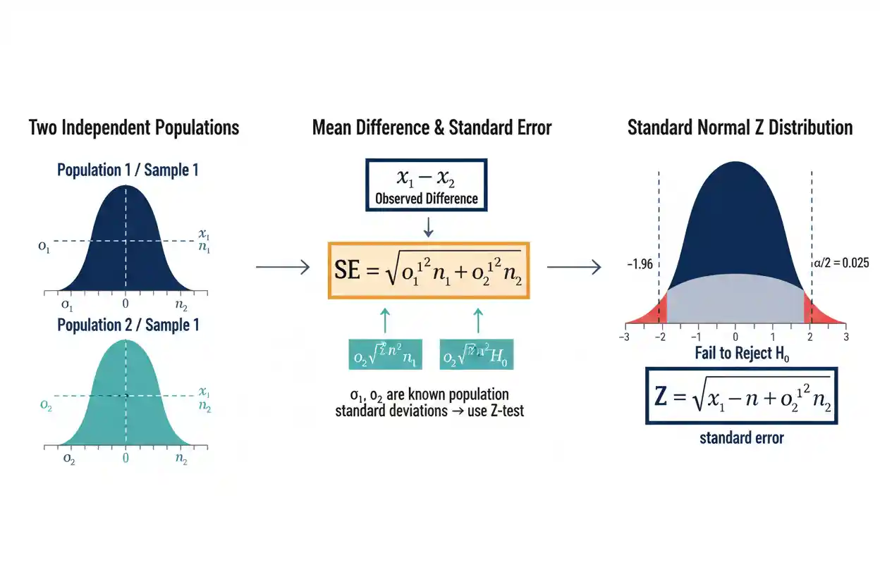

A two-sample z-test is a hypothesis-testing procedure used to compare two independent population means when the population standard deviations are known, or when another justified asymptotic framework produces a statistic with an approximately standard normal reference distribution. In its classical form, the test evaluates whether an observed difference between two independent sample means is large relative to the sampling variability expected under a specified null hypothesis. The most common null hypothesis states that the two population means are equal, although any specified population mean difference can be tested.
Unlike the Two-Sample T-Test, which estimates unknown population variability from the samples and uses a Student’s t reference distribution, the classical two-sample z-test treats σ₁ and σ₂ as known population quantities. The resulting standardized statistic is compared with the standard normal distribution, whose critical values do not depend on degrees of freedom. A statistically significant z-test can provide evidence that the population means differ, but it does not establish practical importance, causation, or the probability that the null hypothesis is true. Correct interpretation also requires genuinely independent sampling units, an appropriate quantitative outcome, a valid standard-error model, and a sampling process that supports the intended inference.
The two-sample z-test is part of Statistics & Probability and the broader Inference & Regression framework. Its defining feature is the use of a standard normal reference distribution for comparing two independent population quantities.
What Is a Two-Sample Z-Test?
Suppose two independent populations have means:
μ₁
and:
μ₂
Samples from those populations produce means:
x̄₁
and:
x̄₂
The observed difference is:
x̄₁ − x̄₂
A common hypothesis test is:
H₀: μ₁ − μ₂ = 0
against:
H₁: μ₁ − μ₂ ≠ 0
The two-sample z-test asks whether the sample mean difference is sufficiently far from zero relative to the standard error expected under the sampling model.
More generally:
H₀: μ₁ − μ₂ = Δ₀
where:
Δ₀
is the hypothesized population mean difference.
The test statistic has the structure:
z = (observed difference − hypothesized difference) / standard error
For two independent means with known population variances:
z = [(x̄₁ − x̄₂) − Δ₀] / √(σ₁²/n₁ + σ₂²/n₂)
This formula is the core of the classical two-sample z-test.
Two-Sample Z-Test Formula
The standard formula is:
z = [(x̄₁ − x̄₂) − Δ₀] / √(σ₁²/n₁ + σ₂²/n₂)
where:
- x̄₁ = Sample 1 mean
- x̄₂ = Sample 2 mean
- μ₁ = Population 1 mean
- μ₂ = Population 2 mean
- Δ₀ = hypothesized population mean difference
- σ₁ = known population standard deviation for Population 1
- σ₂ = known population standard deviation for Population 2
- n₁ = Sample 1 size
- n₂ = Sample 2 size
For the common equal-means null:
H₀: μ₁ = μ₂
we have:
Δ₀ = 0
so the formula simplifies to:
z = (x̄₁ − x̄₂) / √(σ₁²/n₁ + σ₂²/n₂)
The denominator is the standard error of the independent sample mean difference.
Standard Error of the Difference
For independent sample means:
Var(x̄₁) = σ₁²/n₁
and:
Var(x̄₂) = σ₂²/n₂
Because the samples are independent:
Var(x̄₁ − x̄₂) = Var(x̄₁) + Var(x̄₂)
Therefore:
Var(x̄₁ − x̄₂) = σ₁²/n₁ + σ₂²/n₂
Taking the square root gives:
SE(x̄₁ − x̄₂) = √(σ₁²/n₁ + σ₂²/n₂)
This standard error measures the amount of sample-to-sample variation expected in the difference between sample means.
A larger standard error means the observed difference is estimated less precisely.
A smaller standard error means the difference is estimated more precisely.
Why the Variances Are Added
The variance of a difference between random variables is generally:
Var(X − Y) = Var(X) + Var(Y) − 2Cov(X,Y)
For independent samples:
Cov(x̄₁,x̄₂) = 0
Therefore:
Var(x̄₁ − x̄₂) = Var(x̄₁) + Var(x̄₂)
The variances add even though the sample means are being subtracted.
This often seems counterintuitive at first, but uncertainty from both estimates contributes to uncertainty in their difference.
The subtraction applies to the means themselves; the independent uncertainty contributions still accumulate.
Worked Two-Sample Z-Test Example
Suppose two independent production systems are compared using a quantitative output score.
Population 1 has known standard deviation:
σ₁ = 10
Population 2 has known standard deviation:
σ₂ = 12
A sample from Population 1 gives:
n₁ = 64
x̄₁ = 105
A sample from Population 2 gives:
n₂ = 81
x̄₂ = 100
The question is whether the population means differ.
Use:
H₀: μ₁ − μ₂ = 0
and:
H₁: μ₁ − μ₂ ≠ 0
The observed difference is:
x̄₁ − x̄₂ = 105 − 100
= 5
Step 1: Calculate the First Variance Component
For Population 1:
σ₁²/n₁ = 10²/64
= 100/64
= 1.5625
Step 2: Calculate the Second Variance Component
For Population 2:
σ₂²/n₂ = 12²/81
= 144/81
≈ 1.7778
Step 3: Calculate the Standard Error
Add the variance components:
1.5625 + 1.7778
≈ 3.3403
Take the square root:
SE = √3.3403
SE ≈ 1.828
Therefore:
SE(x̄₁ − x̄₂) ≈ 1.83
The observed five-unit sample mean difference is estimated with a standard error of approximately 1.83 units.
Step 4: Calculate the Z Statistic
The null difference is:
Δ₀ = 0
Therefore:
z = (5 − 0) / 1.828
z ≈ 2.735
The observed mean difference lies approximately:
2.74 standard errors
above the zero-difference null value.
Step 5: Find the P-Value
For a two-sided standard normal test:
z ≈ 2.735
The corresponding two-sided p-value is approximately:
p ≈ 0.0062
Suppose the chosen significance threshold is:
α = 0.05
Because:
0.0062 < 0.05
the result falls inside the rejection region.
The decision is:
Reject H₀
The data provide statistical evidence that the two population means differ under the assumptions of the two-sample z-test.
Confidence Interval for the Mean Difference
The corresponding confidence interval for:
μ₁ − μ₂
when population standard deviations are known is:
(x̄₁ − x̄₂) ± z* × √(σ₁²/n₁ + σ₂²/n₂)
For a 95% confidence interval:
z* ≈ 1.96
The estimated difference is:
5
and:
SE ≈ 1.828
The margin of error is:
1.96 × 1.828
≈ 3.583
Therefore:
Lower limit ≈ 5 − 3.583
≈ 1.417
and:
Upper limit ≈ 5 + 3.583
≈ 8.583
The approximate 95% confidence interval is:
1.42 to 8.58
Because zero is outside the interval, the result is consistent with rejecting the corresponding two-sided zero-difference null at α = 0.05.
How to Interpret the Confidence Interval
The sample estimates that Population 1’s mean is:
5 units
higher than Population 2’s.
The interval:
approximately 1.42 to 8.58
communicates uncertainty around that difference.
A conventional frequentist 95% confidence interval does not mean there is a 95% posterior probability that the already-fixed population difference lies inside this particular realized interval.
Instead, the confidence procedure is designed to cover the true parameter in approximately 95% of repeated samples under the assumptions.
The interval provides more information than the hypothesis-test decision alone because it displays plausible magnitudes of the difference.
Critical Values
A z-test compares the observed statistic with critical values from:
Z ∼ Normal(0,1)
For a two-sided test with:
α = 0.05
the critical values are approximately:
−1.96 and +1.96
The rejection rule is:
Reject H₀ if |z| > 1.96
For the example:
|2.735| > 1.96
so H₀ is rejected.
For:
α = 0.01
the two-sided critical values are approximately:
±2.576
Since:
2.735 > 2.576
the worked example would also reject H₀ at the 1% level.
One-Sided Two-Sample Z-Test
Suppose the research question asks whether:
μ₁ > μ₂
A right-tailed test can use:
H₀: μ₁ − μ₂ ≤ 0
H₁: μ₁ − μ₂ > 0
At:
α = 0.05
the standard normal critical value is approximately:
zcritical = 1.645
The decision rule becomes:
Reject H₀ if z > 1.645
The worked example gives:
z ≈ 2.735
so it would reject H₀ in the specified positive direction.
A one-sided test should be selected from the research question before examining which sample mean happens to be larger.
Left-Sided Test
Suppose instead the alternative is:
H₁: μ₁ − μ₂ < 0
The rejection region lies in the lower tail.
At:
α = 0.05
the critical value is approximately:
−1.645
The decision rule is:
Reject H₀ if z < −1.645
A large positive z statistic would not support this left-sided alternative.
Directional testing therefore depends on both magnitude and sign.
Two-Sided Test
A two-sided test evaluates departures in either direction:
H₀: μ₁ − μ₂ = 0
H₁: μ₁ − μ₂ ≠ 0
At:
α = 0.05
the rejection probability is divided equally between both tails:
0.025 in the lower tail
and:
0.025 in the upper tail
The rejection boundaries are:
±1.96
A two-sided test is appropriate when either a positive or negative population difference would be relevant.
It should not be converted into a one-sided test after seeing the observed direction simply to obtain a smaller p-value.
Two-Sample Z-Test vs Two-Sample T-Test
The Two-Sample T-Test and two-sample z-test have similar structures.
Classical two-sample z-test:
z = [(x̄₁ − x̄₂) − Δ₀] / √(σ₁²/n₁ + σ₂²/n₂)
Welch two-sample t-test:
t = [(x̄₁ − x̄₂) − Δ₀] / √(s₁²/n₁ + s₂²/n₂)
The crucial difference is:
z-test uses σ₁ and σ₂
while:
t-test uses s₁ and s₂
The z-test treats the population standard deviations as known.
The t-test estimates them from the samples and uses a Student’s t distribution to account for the resulting uncertainty.
Known Population Standard Deviations
The classical z formula assumes that:
σ₁
and:
σ₂
are known population quantities.
This situation is less common in ordinary research than textbook examples can suggest.
Population standard deviations might be considered known when a measurement process has extremely well-established variance from extensive historical calibration or when the statistical model specifies the variance externally.
If the only available variability estimates are:
s₁ and s₂
calculated from the current samples, a two-sample t procedure is generally the natural classical approach.
Simply having a large n does not transform sample standard deviations into known population parameters.
Does a Large Sample Automatically Mean Use Z?
No.
A common shortcut says:
large sample → z-test
small sample → t-test
This is an oversimplification.
In the classical mean-testing distinction, the important question is whether population standard deviations are treated as known or estimated.
If σ₁ and σ₂ are unknown, using a t procedure remains statistically coherent even with large samples.
As sample sizes grow, t critical values approach z critical values, so numerical results may become very similar.
But similarity does not mean the unknown standard deviations have become conceptually known.
Why T and Z Become Similar in Large Samples
Student’s t distributions have heavier tails than the standard normal distribution.
The amount of additional tail weight decreases as degrees of freedom increase.
As:
df → ∞
the t distribution approaches:
Normal(0,1)
Therefore, a large-sample Welch t-test may produce results extremely close to those of a z approximation.
For example, a 95% two-sided t critical value may approach:
1.96
as degrees of freedom become large.
This convergence explains numerical similarity without eliminating the conceptual distinction between known and estimated variance.
Independent Samples Requirement
The two-sample z formula:
SE = √(σ₁²/n₁ + σ₂²/n₂)
assumes the two sample means are independent.
If observations are paired, the covariance between them matters.
For dependent sample means:
Var(x̄₁ − x̄₂)
contains a covariance term rather than simply the sum of two independent variance components.
Examples of dependent data include:
- before-and-after measurements from the same people
- matched twins
- deliberately matched observational units
- repeated measurements
Using an independent-samples z formula for paired data can misrepresent uncertainty.
Independence Within Samples
The observations inside each group should also provide the independence assumed by the standard-error formula.
Suppose Group 1 contains 200 measurements collected from ten people, with 20 observations from each person.
Those measurements may be strongly correlated within individuals.
Treating them as 200 independent observations can make:
σ₁²/n₁
far too small as a representation of sampling uncertainty.
Clustered, repeated, spatial, or time-dependent observations require a sampling model that reflects their covariance structure.
The row count alone does not determine effective information.
Random Sampling and Generalization
A z-test can calculate a statistic for any numerical dataset, but population inference requires a defensible sampling process.
A random or appropriately designed sample supports generalization to the target population under corresponding assumptions.
A convenience sample may produce an extremely small standard error while remaining systematically unrepresentative.
Increasing n reduces random sampling variability within the mechanism that generated the data.
It does not automatically correct:
- selection bias
- measurement bias
- nonresponse bias
- confounding
- poor target-population definition
Precision and representativeness are different properties.
Normality and the Z-Test
If the population observations are normally distributed and σ values are known, the sample means are exactly normally distributed under independent sampling.
If the populations are non-normal, sufficiently well-behaved large samples can make the sample mean difference approximately normal through central-limit behavior.
However, there is no universal sample-size cutoff guaranteeing an adequate approximation.
Severe skewness, heavy tails, unusual dependence, or distributions without suitable finite variance can complicate normal approximation.
The relevant question is whether the sampling distribution of:
x̄₁ − x̄₂
is adequately represented by the normal model used for the test.
No Universal n = 30 Rule
The claim:
n ≥ 30 means z-tests are valid
is not a mathematical guarantee.
If both underlying populations are normal, sample means can be normally distributed with much smaller n.
If one population is extremely heavy-tailed or strongly skewed, 30 observations may be insufficient for a good normal approximation.
If observations are correlated, even thousands of rows can fail to provide the effective information assumed by an independent-sample formula.
A valid test depends on the actual sampling distribution, not on one memorized threshold.
Testing a Nonzero Mean Difference
The two-sample z-test does not require:
Δ₀ = 0
Suppose a process benchmark states that Population 1 should exceed Population 2 by exactly:
3 units
Then:
H₀: μ₁ − μ₂ = 3
The statistic is:
z = [(x̄₁−x̄₂)−3] / SE
If the observed mean difference is:
5
then the numerator is:
5 − 3 = 2
The test asks whether the population difference departs significantly from three, not whether the two means are equal.
The null benchmark should therefore always be clearly specified.
Type I Error
A Type I Error occurs when a test rejects H₀ even though H₀ is true.
For a correctly calibrated simple-null test:
α = P(reject H₀ | H₀ true)
If:
α = 0.05
then the testing procedure is designed to falsely reject the true null about 5% of the time under repeated application and the model assumptions.
This does not mean:
P(H₀ true | significant result) = 0.05
The conditional probability is different.
The z-test controls a procedural error probability, not a posterior probability that the hypothesis is true or false.
Type II Error and Statistical Power
If a specified alternative is true but the test fails to reject H₀, a Type II error has occurred.
Its probability is:
β
The corresponding Statistical Power is:
Power = 1 − β
Power generally increases when:
- the true population difference grows
- sample sizes increase
- population variability decreases
- the significance threshold becomes less restrictive
- the design becomes more statistically efficient
A nonsignificant result in a low-power study can therefore be inconclusive rather than strong evidence that the population means are equal.
Approximate Power Structure
Suppose:
Δ = μ₁ − μ₂
is the true population difference.
The standard error is:
SE = √(σ₁²/n₁ + σ₂²/n₂)
The standardized separation between the null and alternative is approximately:
Δ / SE
As this value becomes larger, the alternative sampling distribution moves farther from the null distribution.
Therefore:
larger |Δ| → greater power
larger n₁ or n₂ → smaller SE → greater power
larger σ₁ or σ₂ → larger SE → lower power
This signal-to-noise relationship explains the main determinants of two-sample z-test sensitivity.
Sample Size and Standard Error
Suppose:
σ₁ = σ₂ = 10
and:
n₁ = n₂ = 25
Then:
SE = √(100/25 + 100/25)
= √8
≈ 2.828
Now increase both group sizes to:
n₁ = n₂ = 100
Then:
SE = √(100/100 + 100/100)
= √2
≈ 1.414
Quadrupling both group sizes halves the standard error.
The same population mean difference will therefore produce approximately twice the absolute z statistic.
Balanced Sample Sizes
When group variances and per-observation costs are similar, balanced sample allocation often provides good precision.
For a fixed total sample:
n₁ + n₂ = N
the quantity:
σ²/n₁ + σ²/n₂
under equal variances is minimized when the samples are balanced.
For example, with:
N = 100
a:
50/50
allocation provides a smaller standard error than a:
90/10
allocation if the variances are equal.
Unequal allocation can still be appropriate when costs, variances, recruitment constraints, or ethical considerations differ.
Statistical Significance vs Practical Importance
Suppose a very large study estimates:
μ₁ − μ₂ ≈ 0.05
with an extremely small standard error.
The result may produce:
|z| > 10
and:
p < 0.001
Yet a difference of 0.05 units may have no meaningful practical consequence.
Conversely, a smaller study may estimate a difference of ten units but have enough uncertainty that:
p > 0.05
Statistical significance concerns the difference relative to sampling uncertainty.
Practical importance concerns the magnitude of the difference in its real-world context.
These are separate questions.
Effect Size
The raw mean difference is:
x̄₁ − x̄₂
and should generally be reported because it retains the original measurement units.
A standardized population difference can also be described relative to an appropriate standard deviation.
For example, if a common reference standard deviation σ is meaningful:
standardized effect = (μ₁ − μ₂)/σ
A five-unit mean difference can represent a large effect on a low-variance scale or a small effect on a highly variable scale.
Standardized effects are therefore useful for scale-free context, while raw effects preserve practical meaning.
Failure to Reject H₀ Does Not Prove Equal Means
Suppose:
z = 0.80
and:
p = 0.42
The test fails to reject:
H₀: μ₁ − μ₂ = 0
This does not prove:
μ₁ = μ₂
The study may simply lack enough precision to distinguish a moderate population difference from zero.
A confidence interval can clarify this.
If the interval is:
−20 to 25
the data remain compatible with substantial differences in either direction.
If the objective is to demonstrate that the means are sufficiently similar within a predefined tolerance, an equivalence procedure is more appropriate than an ordinary nonsignificant z-test.
Two-Sample Z-Test and Two-Way ANOVA
A Two-Way Anova addresses a factorial design involving two explanatory factors and can evaluate main effects and interactions.
The two-sample z-test instead owns a much narrower question:
comparison of two independent population means under a z-based sampling framework
If a study contains only:
Group A vs Group B
one two-group comparison may be sufficient.
If the design contains factors such as:
Treatment × Region
or:
Method × Experience Level
a factorial model can address whether the effect of one factor changes across levels of the other.
Repeated two-sample tests do not automatically reproduce that interaction analysis.
Multiple Comparisons
Suppose four groups are present and researchers perform a two-sample z-test for every pair at:
α = 0.05
The per-comparison Type I error probability may be 5%, but the probability of obtaining at least one false rejection across the entire family can be substantially larger.
This is a multiplicity problem.
The two-sample z-test should therefore be used for a prespecified two-group comparison or within an inferential framework that handles multiple comparisons appropriately.
Adding many unadjusted pairwise tests changes the overall error behavior.
Standardized Residuals vs Z-Test Statistics
Standardized Residuals and z statistics both put quantities on standardized scales, but they answer different questions.
A two-sample z statistic is:
z = [(x̄₁−x̄₂)−Δ₀] / SE
It measures how far an estimated group mean difference lies from its null value in sampling-standard-error units.
A standardized residual measures how far one observed response lies from its fitted model prediction relative to its estimated residual variability.
The first is an inferential statistic concerning a population contrast.
The second is primarily an observation-level model diagnostic.
They should not be interpreted interchangeably.
Z Statistic vs Z-Score
A z-score for an individual observation often has the form:
z = (x − μ)/σ
A two-sample z-test statistic instead standardizes:
a difference between two sample means
using the standard error of that difference.
Although both are called z values because they are interpreted through a standard normal scale, their numerators and denominators represent different statistical quantities.
A z-test statistic of 2.5 does not mean an individual observation lies 2.5 population standard deviations above a mean.
It means the estimated population contrast lies 2.5 standard errors from its hypothesized value.
Two-Sample Z-Test for Proportions
The phrase two-sample z-test is also commonly used for comparing two population proportions.
Suppose two independent samples produce:
p̂₁ = x₁/n₁
and:
p̂₂ = x₂/n₂
A test of:
H₀: p₁ = p₂
uses a z-based sampling framework, but its standard-error formula differs from the known-σ mean formula because binary outcomes have variance related to the underlying proportions.
For the ordinary pooled null test of equal proportions, a pooled estimate:
p̂ = (x₁ + x₂)/(n₁ + n₂)
is used in the null standard error:
SE₀ = √[p̂(1−p̂)(1/n₁ + 1/n₂)]
and:
z = (p̂₁ − p̂₂)/SE₀
This is a distinct application of the z-test principle.
Why Mean and Proportion Formulas Should Not Be Mixed
For two means with known population variances:
SE = √(σ₁²/n₁ + σ₂²/n₂)
For the usual null test of two independent proportions:
SE₀ = √[p̂(1−p̂)(1/n₁ + 1/n₂)]
These formulas arise from different outcome distributions.
Using the mean formula for binary proportions or the pooled-proportion formula for continuous measurements would be incorrect.
The term “two-sample z-test” describes a standard-normal testing framework, but the appropriate standard error must come from the parameter and data model actually being tested.
Two-Proportion Example
Suppose Sample 1 contains:
120 successes out of 200
so:
p̂₁ = 120/200 = 0.60
Sample 2 contains:
90 successes out of 200
so:
p̂₂ = 90/200 = 0.45
The observed difference is:
0.60 − 0.45 = 0.15
Under:
H₀: p₁ = p₂
the pooled proportion is:
p̂ = (120 + 90)/(200 + 200)
= 210/400
= 0.525
The null standard error is:
SE₀ = √[(0.525)(0.475)(1/200 + 1/200)]
≈ √0.002494
≈ 0.0499
Therefore:
z ≈ 0.15/0.0499
z ≈ 3.01
The result would provide strong evidence against equal population proportions under the corresponding test assumptions.
Conditions for the Two-Proportion Normal Approximation
A two-proportion z-test depends on the binomial sampling model and an adequate normal approximation.
The expected counts under the null should be sufficiently large for the approximation to represent the discrete sampling distribution well.
A rigid threshold is not universally optimal, but extremely small expected success or failure counts can make the normal approximation poor.
When samples are small or probabilities are close to boundaries such as 0 or 1, an exact or otherwise better-calibrated procedure may be preferable.
The appropriate method should reflect the actual sampling distribution rather than applying a z formula automatically.
Random Assignment and Causation
Suppose a randomized experiment assigns participants to two treatments and uses a two-sample z framework.
Random assignment can support causal interpretation because treatment allocation is designed to break systematic relationships with pre-treatment confounders in expectation.
By contrast, if participants select their own groups, an observed mean difference can result from pre-existing group differences.
The test statistic itself does not distinguish these situations.
The z-test quantifies uncertainty in the contrast under the specified sampling model.
Causal meaning comes from the study design and assumptions.
Random Sampling and Population Inference
Random assignment helps treatment comparison.
Random sampling helps population generalization.
A study can have one without the other.
For example, a randomized experiment using a convenience sample may support a strong internal causal comparison for the enrolled participants while offering more limited generalizability to a broader population.
A two-sample z-test does not automatically solve this distinction.
The scope of inference should match the design through which observations and treatment conditions were obtained.
Common Two-Sample Z-Test Mistakes
A common mistake is using the z-test simply because both sample sizes are large, even though population standard deviations are unknown and estimated from the same samples. A t procedure remains appropriate in the classical unknown-variance setting.
Another error is using the independent-samples formula for paired data.
Researchers also sometimes interpret:
p < 0.05
as meaning H₀ has less than a 5% probability of being true.
That is incorrect.
Another mistake is assuming statistical significance establishes a practically important difference or causal effect.
For proportion tests, an additional error is using the mean-based standard-error formula or forgetting that the null test and confidence interval may use different proportion standard-error constructions.
Finally, performing many unadjusted two-sample tests across several groups can inflate family-level false-positive risk.
How to Calculate a Two-Sample Z-Test for Means
Start with:
x̄₁, x̄₂, σ₁, σ₂, n₁, n₂
State:
H₀: μ₁ − μ₂ = Δ₀
and the appropriate alternative.
Calculate:
SE = √(σ₁²/n₁ + σ₂²/n₂)
Then:
z = [(x̄₁−x̄₂)−Δ₀]/SE
Use the standard normal distribution to obtain the p-value or compare z with the relevant critical value.
For a two-sided test at:
α = 0.05
reject H₀ when:
|z| > 1.96
Finally, report the estimated mean difference and an appropriate confidence interval rather than reporting the significance decision alone.
How to Report a Two-Sample Z-Test
For the worked example:
Sample 1 mean = 105
Sample 2 mean = 100
Estimated difference = 5
SE ≈ 1.83
z ≈ 2.74
p ≈ 0.006
95% CI ≈ 1.42 to 8.58
A concise interpretation is that Population 1’s mean was estimated to be five units higher than Population 2’s, with the sampling model providing evidence that the population difference is not zero.
The interval should then be used to assess whether the plausible magnitude of that difference is important in the actual application.
Frequently Asked Questions
What is a two-sample z-test?
A two-sample z-test compares two independent population quantities using a statistic whose reference distribution is standard normal. In the classical mean version, population standard deviations are known.
What is the formula for two independent means?
z = [(x̄₁−x̄₂)−Δ₀] / √(σ₁²/n₁ + σ₂²/n₂)
What is usually the null hypothesis?
A common null is:
H₀: μ₁ − μ₂ = 0
What does Δ₀ mean?
Δ₀ is the population mean difference specified by the null hypothesis.
What distribution does the test statistic use?
The standard normal distribution:
Z ∼ Normal(0,1)
under the null framework.
What are the two-sided critical values at α = 0.05?
Approximately:
−1.96 and +1.96
What is the one-sided critical value at α = 0.05?
Approximately:
1.645
for an upper-tail test or:
−1.645
for a lower-tail test.
What is the difference between a two-sample z-test and t-test?
The classical z-test uses known population standard deviations. The t-test estimates population variability from sample data and uses a Student’s t reference distribution.
Does a large sample automatically require a z-test?
No. Large samples make t and z critical values numerically similar, but they do not automatically make unknown population standard deviations known.
Can the two groups have different population variances?
Yes. The known-variance z formula directly uses:
σ₁²/n₁ + σ₂²/n₂
so σ₁ and σ₂ need not be equal.
Do sample sizes have to be equal?
No.
Must the two samples be independent?
Yes for the standard independent two-sample formula.
Can I use this test for before-and-after data?
Not with the ordinary independent-samples formula if the measurements come from the same individuals. Their dependence should be modeled.
Does the data have to be normally distributed?
Exact normal theory follows naturally for normal populations, while large-sample normal approximation can apply more broadly under suitable conditions. There is no universal sample-size threshold guaranteeing adequacy.
Is n = 30 always enough?
No.
What does a positive z statistic mean?
When the contrast is x̄₁ − x̄₂, a positive z means the observed difference lies above the null difference.
Does p < 0.05 mean H₀ has less than a 5% probability of being true?
No.
Does a significant two-sample z-test prove a causal difference?
No. Causal interpretation depends on the study design.
Does a nonsignificant result prove equal population means?
No. It means the test did not provide sufficient evidence against the stated null at the chosen threshold.
Can a two-sample z-test compare proportions?
Yes. A common two-proportion z-test uses a standard-normal framework, but its standard-error formula differs from the continuous-mean formula.
What is the pooled proportion under H₀: p₁ = p₂?
p̂ = (x₁+x₂)/(n₁+n₂)
What is the standard error for the usual pooled two-proportion null test?
SE₀ = √[p̂(1−p̂)(1/n₁+1/n₂)]
How does sample size affect the test?
Larger independent samples reduce standard error and generally increase statistical power.
Is statistical significance the same as practical importance?
No. A tiny effect can be highly statistically significant when estimated very precisely.
Why report a confidence interval?
It shows the estimated magnitude and precision of the population difference instead of reducing the conclusion to a binary testing decision.
Key Takeaway
The two-sample z-test evaluates whether an observed difference between two independent sample estimates is large relative to the sampling variation expected under a specified null hypothesis. For the classical comparison of two means with known population variances:
z = [(x̄₁−x̄₂)−Δ₀] / √(σ₁²/n₁ + σ₂²/n₂)
and for the common equal-means null:
Δ₀ = 0
The resulting statistic is evaluated using the standard normal distribution. At a two-sided significance level of:
α = 0.05
the familiar critical values are approximately:
±1.96
The classical z-test differs from the two-sample t-test because σ₁ and σ₂ are treated as known rather than estimated from the current samples. Large samples can make t and z results numerically similar, but they do not by themselves convert unknown population standard deviations into known quantities.
The term two-sample z-test can also describe z-based comparisons of two population proportions, where the appropriate standard error follows from the binomial model rather than the known-variance mean formula. In every application, the standardization must match the parameter and sampling process being analyzed.
Most importantly, a z-test provides evidence about a specified population contrast relative to sampling uncertainty. It does not establish the probability that the null hypothesis is true, guarantee practical importance, or create causal evidence that is absent from the study design. Reliable interpretation combines the z statistic with the estimated effect, confidence interval, significance threshold, statistical power, sampling assumptions, and the real-world importance of the observed difference.