
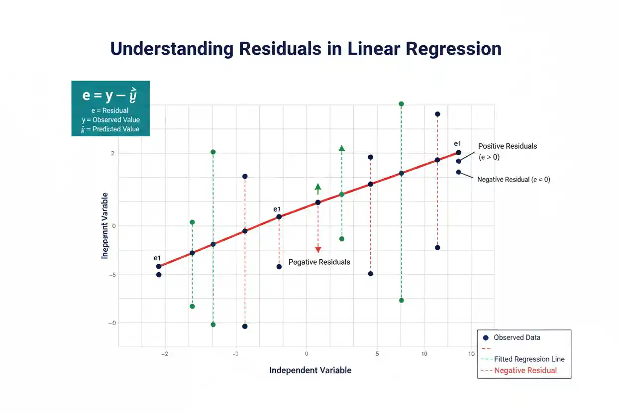

Residuals are the differences between observed values and the values predicted by a fitted statistical model. In regression, each residual measures the vertical prediction error remaining after the model has used its predictors to estimate the response. If an observed value is larger than its prediction, the residual is positive; if the observed value is smaller than its prediction, the residual is negative. Residuals are central to regression because they reveal information that the fitted coefficients alone cannot show. A regression equation can appear reasonable while its residuals reveal curvature, changing variance, dependence, extreme observations, or other evidence that the model does not represent the data adequately.
Ordinary least squares regression is fitted by choosing coefficients that minimize the sum of squared residuals, so residuals also determine the numerical solution of the model. However, a residual is not identical to the unobservable population error term: an error represents deviation from the true population regression function, while a residual is calculated after estimating that function from sample data. This distinction matters for statistical inference because residuals inherit constraints from the fitting process. Proper residual analysis therefore combines simple calculations with graphical patterns, scale, model assumptions, and the purpose of the regression.
Residuals are a foundational topic within Statistics & Probability and Inference & Regression. They connect fitted coefficients such as the Regression Intercept and Regression Slope with the unexplained variation that remains after prediction.
What Are Residuals?
Suppose a regression model produces a predicted response:
ŷᵢ
for an observation whose actual response is:
yᵢ
The residual is:
eᵢ = yᵢ − ŷᵢ
The calculation always follows:
residual = observed value − predicted value
Suppose:
y = 75
and:
ŷ = 70
Then:
e = 75 − 70
e = 5
The model underpredicted the observed response by five units.
If instead:
y = 65
while:
ŷ = 70
then:
e = 65 − 70
e = −5
The model overpredicted the response by five units.
The sign therefore indicates direction, while the absolute value indicates the size of the prediction discrepancy on the response scale.
Residual Formula
The basic residual formula is:
eᵢ = yᵢ − ŷᵢ
For simple linear regression:
ŷᵢ = b₀ + b₁xᵢ
so:
eᵢ = yᵢ − (b₀ + b₁xᵢ)
For multiple linear regression:
ŷᵢ = b₀ + b₁x₁ᵢ + b₂x₂ᵢ + … + bₖxₖᵢ
therefore:
eᵢ = yᵢ − (b₀ + b₁x₁ᵢ + b₂x₂ᵢ + … + bₖxₖᵢ)
Every observation receives its own fitted value and therefore its own residual.
The collection:
e₁, e₂, …, eₙ
contains much of the information used to evaluate how well the fitted model represents the observed responses.
Positive Residuals
A residual is positive when:
yᵢ > ŷᵢ
Suppose:
observed value = 120
predicted value = 112
Then:
e = 120 − 112
e = 8
The observed response lies eight units above the fitted regression value.
On an ordinary regression scatterplot, this observation appears above the regression line.
A positive residual does not mean the observation itself is unusually large in an absolute sense. It means the observation is larger than the value predicted for its particular predictor values.
An observation of 120 could have a small positive residual if the model predicted 119, or an enormous positive residual if the model predicted 40.
Residuals are therefore conditional on the model’s predictions.
Negative Residuals
A residual is negative when:
yᵢ < ŷᵢ
For example:
observed value = 45
predicted value = 52
Then:
e = 45 − 52
e = −7
The regression model overpredicted the observed response by seven units.
Graphically, the point lies below the fitted regression line.
The negative sign does not imply a “bad” observation. Positive and negative residuals are both normal features of a fitted model.
A well-centered regression generally requires residuals on both sides of zero.
Zero Residual
A residual equals zero when:
yᵢ = ŷᵢ
For example:
y = 60
ŷ = 60
gives:
e = 0
The model predicts that particular observation exactly.
A regression model does not need every residual to equal zero to be useful. In most real datasets, unexplained variation remains even when the systematic relationship is modeled well.
If every residual were exactly zero, the model would fit every observed response perfectly. Such a fit can occur in special deterministic settings or highly parameterized models, but in ordinary noisy data it may also raise questions about overfitting or data structure.
Worked Residual Example
Consider the following observations:
| x | y |
|---|---|
| 1 | 2 |
| 2 | 4 |
| 3 | 5 |
| 4 | 8 |
| 5 | 11 |
Suppose ordinary least squares produces the fitted regression:
ŷ = −0.6 + 2.2x
At:
x = 1
the predicted value is:
ŷ = −0.6 + 2.2(1)
ŷ = 1.6
The observed value is:
y = 2
so:
e = 2 − 1.6
e = 0.4
The first observation has a positive residual of 0.4.
Calculate Every Residual
For x = 2:
ŷ = −0.6 + 2.2(2)
ŷ = 3.8
Therefore:
e = 4 − 3.8
e = 0.2
For x = 3:
ŷ = −0.6 + 2.2(3)
ŷ = 6.0
Therefore:
e = 5 − 6
e = −1.0
For x = 4:
ŷ = −0.6 + 2.2(4)
ŷ = 8.2
Therefore:
e = 8 − 8.2
e = −0.2
For x = 5:
ŷ = −0.6 + 2.2(5)
ŷ = 10.4
Therefore:
e = 11 − 10.4
e = 0.6
The residuals are therefore:
0.4, 0.2, −1.0, −0.2, 0.6
Sum of Residuals
Add the residuals:
Σeᵢ = 0.4 + 0.2 − 1.0 − 0.2 + 0.6
Σeᵢ = 0
This is not an accident.
For ordinary least squares regression that includes an estimated intercept:
Σeᵢ = 0
apart from numerical rounding.
Consequently:
ē = 0
where ē is the mean residual.
This property arises from the mathematical conditions used to minimize the residual sum of squares.
It does not mean every individual residual is small. Large positive and negative residuals can still sum to zero.
Why OLS Residuals Sum to Zero
Ordinary least squares minimizes:
SSE = Σeᵢ²
For simple regression:
SSE = Σ[yᵢ − (b₀ + b₁xᵢ)]²
When this expression is minimized with respect to the intercept b₀, one of the resulting normal equations is:
Σ[yᵢ − (b₀ + b₁xᵢ)] = 0
But the expression inside the summation is simply:
eᵢ
so:
Σeᵢ = 0
This property depends on the ordinary model containing an intercept.
A model deliberately fitted without an intercept does not generally have residuals that sum to zero.
Residuals vs Errors
Residual and error are related terms but are not strictly identical.
The population regression model can be written:
Yᵢ = β₀ + β₁Xᵢ + εᵢ
The population error is:
εᵢ = Yᵢ − E(Yᵢ | Xᵢ)
It describes the deviation of an observation from the true population regression function.
The problem is that β₀ and β₁ are usually unknown. Therefore the true error εᵢ cannot normally be observed directly.
After estimating the regression from sample data, we calculate:
eᵢ = yᵢ − ŷᵢ
The residual eᵢ is therefore an observable estimate-related counterpart of the unobservable population error εᵢ.
Why Residuals and Errors Differ
Suppose the true population relationship is:
Y = 10 + 3X + ε
but a particular sample produces the estimated regression:
ŷ = 11 + 2.8x
For an observation at x = 5 with y = 24:
the population conditional mean is:
E(Y | X = 5) = 10 + 3(5)
= 25
so the true error is:
ε = 24 − 25
ε = −1
The fitted sample prediction is:
ŷ = 11 + 2.8(5)
ŷ = 25
which happens to give the same value in this example, but generally it will differ from the true regression mean.
The residual therefore combines the observation’s underlying random error with uncertainty created by estimating the regression coefficients.
Residual Sum of Squares
The residual sum of squares is:
SSE = Σeᵢ²
It can also be written:
SSE = Σ(yᵢ − ŷᵢ)²
Using the worked residuals:
0.4, 0.2, −1.0, −0.2, 0.6
their squared values are:
0.16, 0.04, 1.00, 0.04, 0.36
Therefore:
SSE = 0.16 + 0.04 + 1 + 0.04 + 0.36
SSE = 1.60
Ordinary least squares chooses the fitted coefficients that make this sum as small as possible among models of the specified linear form.
SSE therefore plays a central role in both estimation and measures of remaining variation.
Why Residuals Are Squared
Simply adding raw residuals is not useful for measuring overall model error because positive and negative values can cancel.
In an OLS model with an intercept:
Σeᵢ = 0
regardless of whether the individual residuals are tiny or enormous.
Taking absolute values would avoid cancellation, but ordinary least squares instead uses squares:
eᵢ²
Squaring makes all contributions nonnegative and gives relatively greater influence to larger errors.
For example:
residual = 2 → squared residual = 4
while:
residual = 10 → squared residual = 100
The second residual is five times larger in absolute terms but contributes 25 times as much squared error.
Mean Squared Error in Regression
For an ordinary regression with p estimated parameters, the residual mean square is commonly:
MSE = SSE / (n − p)
In simple linear regression with an intercept and one slope:
p = 2
so:
MSE = SSE / (n − 2)
Using the worked example:
SSE = 1.60
n = 5
Therefore:
MSE = 1.60 / (5 − 2)
MSE = 1.60 / 3
MSE ≈ 0.533
The denominator uses residual degrees of freedom rather than simply n because model parameters were estimated from the same observations.
Residual Standard Error
The residual standard error is:
sₑ = √MSE
or in simple regression:
sₑ = √[SSE / (n − 2)]
Using:
MSE ≈ 0.533
gives:
sₑ = √0.533
sₑ ≈ 0.730
This quantity estimates the typical scale of residual variation around the fitted regression relationship under the conventional model.
Because it is expressed in the same units as Y, it can often be interpreted more naturally than SSE.
If Y is measured in dollars, sₑ is measured in dollars. If Y is measured in seconds, sₑ is measured in seconds.
Residuals and Fitted Values
A residual-vs-fitted plot places:
fitted value ŷᵢ
on the horizontal axis and:
residual eᵢ
on the vertical axis.
The horizontal reference line is:
e = 0
A well-specified linear mean model with approximately constant variance should generally produce residuals scattered around zero without a strong systematic pattern.
The objective is not to make the plot look perfectly random in every finite sample. Some visual irregularity is inevitable.
Instead, analysts look for persistent structures that suggest the fitted model is missing important features of the data.
Curved Residual Pattern
Suppose a residual plot forms a clear U shape:
positive residuals at low fitted values
negative residuals in the middle
positive residuals again at high fitted values
This suggests the fitted linear relationship may be missing curvature.
The model systematically underpredicts in some regions and overpredicts in others.
Adding more observations to the same incorrect straight-line specification may make the pattern even clearer rather than fixing it.
A transformation, polynomial term, spline, or different model may better represent the conditional mean.
Residual analysis therefore helps diagnose functional-form problems.
Funnel-Shaped Residual Pattern
Suppose residuals are tightly clustered around zero for low fitted values but increasingly spread out as fitted values rise.
The resulting plot resembles a funnel.
This suggests:
Var(ε | X)
may not be constant.
The condition is commonly called heteroscedasticity.
Ordinary least squares can still produce fitted coefficients, but conventional constant-variance standard errors and prediction intervals may not accurately represent uncertainty.
The appropriate response depends on why the variance changes and what the analysis is trying to achieve.
Residuals and Constant Variance
A classical linear regression model often assumes:
Var(εᵢ | X) = σ²
This means the conditional error variance is constant across predictor values.
Residuals are used to assess whether the observed data are broadly consistent with that assumption.
If residual magnitude increases systematically with X or fitted values, constant variance may be questionable.
If the spread is broadly similar across the fitted range, the assumption becomes more plausible, although a residual plot can never prove it exactly.
The distinction matters because uncertainty calculations frequently rely on the variance model.
Residuals and Independence
Residuals can also reveal dependence.
Suppose data are ordered by time and the residual sequence is:
positive, positive, positive, positive, negative, negative, negative, negative
Repeated runs of similar signs may indicate serial correlation or unmodeled temporal structure.
If ordinary regression assumes independent errors while actual errors are strongly correlated, conventional standard errors and inferential conclusions can become unreliable.
Residuals should therefore sometimes be plotted against:
time
observation order
geographic location
cluster membership
or another variable that reflects the sampling structure.
The appropriate diagnostic depends on how the observations were generated.
Residuals and Sampling Distribution
A residual is calculated for an individual observed response, while a Sampling Distribution describes how a statistic behaves across repeated samples.
The two concepts should not be confused.
For example, the fitted slope b₁ varies from sample to sample and therefore has a sampling distribution.
Each sample also produces its own set of residuals because both the observations and the fitted coefficients change.
Statistical inference uses assumptions about the underlying errors and sampling process to derive distributions for estimated coefficients and test statistics.
Residuals help assess whether the observed sample behaves consistently with those assumptions, but the empirical residual distribution itself is not automatically the sampling distribution of a coefficient.
Residual Normality
In the classical normal-error linear regression model:
εᵢ ∼ Normal(0, σ²)
conditional on the predictors.
This assumption supports exact finite-sample t and F inference under the rest of the classical conditions.
Analysts often examine residual histograms or quantile-based plots as diagnostics because the true errors cannot be observed directly.
Residuals do not form a perfectly independent sample from the error distribution, however, because they are constrained by the fitted model.
Normality diagnostics should therefore be interpreted approximately rather than treating the residual histogram as a direct observation of the population error density.
Normality Is Not Required to Fit OLS
Ordinary least squares coefficients can be calculated without normally distributed errors.
Normality is primarily connected with particular exact finite-sample inferential results rather than with the arithmetic existence of the fitted line.
A regression can therefore have meaningful OLS coefficient estimates even if residuals are not perfectly normal.
However, severe heavy tails, extreme skewness, or unusual observations can affect finite-sample inference and make mean-based regression summaries unstable.
With large samples, some coefficient inference can rely on asymptotic approximations under weaker conditions, but sample size does not repair every form of model misspecification or dependence.
Residuals and Outliers
An observation with a large residual has a response that is far from its fitted value.
Suppose:
y = 100
ŷ = 40
Then:
e = 60
If most residuals are within ±5, this observation is unusual in the response direction.
However, a large raw residual does not automatically mean the observation has high influence on the regression coefficients.
Influence depends on both residual size and the observation’s predictor position.
A point near the center of the predictor data can have a large residual while exerting relatively limited leverage over the fitted slope.
Residuals vs Leverage
Leverage concerns how unusual an observation’s predictor values are.
An observation can have high leverage even with a small residual.
Imagine nearly all x-values lie between:
0 and 10
while one observation has:
x = 100
If that distant point lies close to the fitted regression line, its residual may be small, yet it can strongly affect the slope because of its unusual predictor location.
Conversely, an observation near x̄ can have a large residual but low leverage.
Residual size and leverage therefore measure different aspects of an observation.
Both matter when evaluating influence.
Raw Residuals and Scale
Raw residuals are measured in the units of Y.
This makes them easy to interpret but difficult to compare across observations when their expected variability differs.
A residual of:
10
may be enormous in one region of a dataset and ordinary in another.
For this reason, regression diagnostics often rescale residuals by an estimate of their standard deviation.
Standardized or studentized forms help identify observations whose errors are large relative to their expected residual variability.
Even when such scaled diagnostics are used, the raw residual remains the underlying observed-minus-predicted difference.
Residuals and the Regression Intercept
The Regression Intercept affects every fitted value:
ŷᵢ = b₀ + b₁xᵢ
and therefore every residual:
eᵢ = yᵢ − b₀ − b₁xᵢ
If the intercept is shifted upward while the slope remains unchanged, all fitted values increase and all residuals decrease by the same amount.
In ordinary OLS with an estimated intercept, the fitting process chooses b₀ partly so that:
Σeᵢ = 0
This centering property disappears in general when a regression is forced through the origin.
The decision to omit an intercept therefore changes the residual structure as well as the coefficient estimates.
Residuals and Regression Slope
The Regression Slope determines how predictions change across values of X.
If the fitted slope is too shallow relative to the systematic data pattern, residuals may tend to be negative at low X and positive at high X.
If it is too steep, the sign pattern may reverse.
Ordinary least squares selects the slope jointly with the intercept to minimize:
Σeᵢ²
A residual plot can then reveal whether one constant slope adequately captures the conditional mean relationship.
A clear residual trend against X indicates that the fitted slope structure may be incomplete.
Residuals and Prediction Intervals
A Prediction Interval accounts for the variability of future observations around their fitted regression mean.
The residual standard error:
sₑ
is a key ingredient in the classical prediction interval formula.
When residual variation is large, prediction intervals become wider because individual future outcomes are less predictable around the fitted relationship.
When residual variation is small, future observations tend to remain closer to their expected regression values, allowing narrower intervals.
However, the classical interval also assumes the residual variance structure has been modeled appropriately.
A small sₑ does not guarantee reliable prediction if the model is misspecified or extrapolated far beyond the observed predictor range.
Residuals and Statistical Significance
Residual variability directly affects the standard errors of regression coefficients.
Greater unexplained variability generally means less precise estimates of intercepts and slopes, other factors held constant.
Less precise coefficients produce smaller test statistics for a given coefficient magnitude and therefore make it harder to cross a chosen Significance Level.
This does not mean residuals themselves determine whether a relationship is important.
A very large sample can produce statistically significant coefficients despite substantial residual variation, while a small sample can contain a meaningful apparent slope that remains statistically uncertain.
Residual scale, coefficient magnitude, sample size, and predictor variation all contribute to inference.
Small Residuals Do Not Automatically Mean a Good Model
A model can produce small residuals in the fitting sample yet perform poorly on new data.
This occurs when the model overfits sample-specific noise.
For example, a sufficiently flexible model can pass extremely close to every observed data point, producing:
eᵢ ≈ 0
for the training sample.
But if that flexibility captures random idiosyncrasies rather than stable structure, predictions for new observations can deteriorate.
Residual fit should therefore be evaluated together with model complexity and out-of-sample validation when prediction is the goal.
Training residuals alone measure in-sample fit.
Large Residuals Do Not Always Mean the Model Is Useless
Some outcomes contain substantial irreducible variability.
Suppose a regression predicts individual spending behavior. Even a useful model may leave large residuals because individual decisions depend on many unobserved factors.
The important questions are whether the model improves prediction relative to meaningful alternatives, whether its residual patterns reveal systematic misspecification, and whether its predictive uncertainty is honestly represented.
A model with residual standard error of 20 is neither inherently good nor bad without knowing the response scale and application.
Residual magnitude must be interpreted contextually.
Residuals in Multiple Regression
For multiple regression:
ŷᵢ = b₀ + b₁x₁ᵢ + b₂x₂ᵢ + … + bₖxₖᵢ
the residual remains:
eᵢ = yᵢ − ŷᵢ
The interpretation is unchanged: it is the observed response minus the predicted response for that complete predictor profile.
Residual diagnostics can be plotted against fitted values or individual predictors to reveal model deficiencies.
For example, residual curvature against X₂ can indicate that the relationship involving X₂ is inadequately modeled even when the overall residual-vs-fitted plot appears relatively unremarkable.
Multiple regression therefore often requires examining residuals from several perspectives.
Residual Degrees of Freedom
In a regression with:
n observations
and:
p estimated parameters
the ordinary residual degrees of freedom are:
dfresidual = n − p
For simple regression with an intercept:
p = 2
so:
dfresidual = n − 2
For a model with an intercept plus five slopes:
p = 6
so:
dfresidual = n − 6
These degrees of freedom appear in variance estimation:
MSE = SSE / (n − p)
Estimating more parameters uses more degrees of freedom, which is one reason model complexity matters when estimating residual variance.
Residuals in a Mean-Only Model
Consider an intercept-only model:
ŷᵢ = ȳ
Every residual is:
eᵢ = yᵢ − ȳ
The residual sum of squares is therefore:
Σ(yᵢ − ȳ)²
which is the total sum of squares around the sample mean.
Adding predictors can reduce SSE by allowing fitted values to vary systematically across observations.
This provides the basis for comparing a regression model with the mean-only baseline.
Residual reduction is therefore central to common measures of regression fit.
Residuals and R²
In ordinary OLS regression with an intercept:
R² = 1 − SSE / SST
where:
SSE = Σeᵢ²
and:
SST = Σ(yᵢ − ȳ)²
A smaller SSE relative to SST produces a larger R².
If:
SSE = 20
and:
SST = 100
then:
R² = 1 − 20/100
R² = 0.80
The regression accounts for 80% of the observed sum-of-squares variation relative to the mean-only baseline.
However, R² compresses the entire residual structure into one number. Two models with similar R² can have very different residual patterns and therefore very different adequacy.
Why Residual Plots Add Information Beyond R²
Suppose two models both have:
R² = 0.90
Model A has residuals scattered without a strong pattern around zero.
Model B has a clear U-shaped residual pattern.
Although their R² values are identical, Model B appears to miss systematic nonlinear structure.
Similarly, a model can have high R² while displaying strongly increasing residual variance.
Residual diagnostics therefore reveal model problems that aggregate fit statistics can conceal.
A regression model should not be judged solely by how much variance it appears to explain.
Residuals and Model Misspecification
Systematic residual structure can indicate that important aspects of the data-generating relationship have not been modeled.
Potential signals include:
- curvature
- changing variance
- clusters or groups
- temporal patterns
- unusually large residuals
- abrupt structural shifts
These patterns do not diagnose their own cause automatically.
For example, a curved pattern might reflect a missing nonlinear term, an omitted variable, a transformation issue, or a mixture of different populations.
Residual analysis identifies where the model is inadequate; substantive reasoning and further analysis are needed to determine why.
Residuals and Omitted Variables
Suppose a regression predicts sales using price alone.
Residuals may display a clear seasonal pattern:
mostly positive in one season
mostly negative in another
This suggests the model systematically underpredicts and overpredicts during different periods.
Season or another related variable may be missing from the model.
Adding an appropriate predictor can reduce this residual structure if the effect is real and stable.
However, the presence of residual patterns does not tell the analyst exactly which omitted variable should be added.
Diagnostics should guide investigation rather than become an automatic variable-selection rule.
Residuals and Transformation
Sometimes residual spread or curvature suggests that the original measurement scale does not fit the assumed linear model well.
A transformation of Y or X may stabilize variance or make the mean relationship more linear.
For example, a response whose variability grows proportionally with its level may sometimes be modeled more effectively on a logarithmic scale.
After transforming the response, however, residuals are measured on that transformed scale.
Interpretation of model errors and predictions on the original scale then requires care because nonlinear transformations do not preserve differences and expectations in a simple one-to-one linear manner.
Residuals in Time-Ordered Data
For observations collected over time, residual order contains information that an ordinary residual-vs-fitted plot may miss.
Suppose consecutive residuals repeatedly alternate:
positive, negative, positive, negative
or occur in long same-sign runs.
Such patterns can indicate temporal dependence or an omitted trend or seasonal component.
A standard independent-error regression assumes that residual-like errors do not contain systematic serial dependence after the modeled structure has been removed.
When this assumption fails, time-series or correlated-error methods may be more appropriate.
Residual Diagnostics Are Not Formal Proof
Residual plots are valuable but involve judgment.
A random sample can produce apparent patterns even when the model assumptions hold, while a small dataset may hide genuine violations.
Formal tests exist for certain residual properties, but they also have limitations. Large samples can make trivial deviations statistically detectable, while small samples may lack power to detect important departures.
Diagnostic interpretation should therefore combine graphical evidence, statistical procedures, domain knowledge, and sensitivity analysis rather than treating any single rule as definitive.
Why Residual Sign Alone Is Not Enough
A model with approximately equal numbers of positive and negative residuals can still be badly misspecified.
Consider a U-shaped pattern in which residuals are positive at low and high X values but negative in the middle.
Positive and negative errors may balance perfectly:
Σeᵢ = 0
while the model systematically misses the true relationship.
The fact that OLS residuals sum to zero is therefore not evidence that the regression fits well.
What matters is whether residual magnitude and structure are compatible with the model’s intended assumptions and use.
Comparing Residuals Across Models
Raw residuals can be compared directly when competing models predict the same response variable for the same observations.
A lower SSE indicates better in-sample least-squares fit.
However:
lower SSE ≠ automatically better model
A more complex model can nearly always reduce training SSE by adding enough flexibility.
Model comparison should also account for complexity, inferential purpose, validation performance, and whether the added structure is substantively justified.
For predictive tasks, residuals on held-out observations can provide more realistic information about generalization than training residuals alone.
Common Residual Mistakes
A frequent mistake is reversing the residual formula. The standard convention is:
observed − predicted
not:
predicted − observed
Another error is calling residuals and population errors exactly the same thing. Errors belong to the unknown population model, while residuals are calculated from fitted sample predictions.
Researchers also sometimes assume that residuals summing to zero proves a good fit. In OLS with an intercept, that result is an algebraic property regardless of whether the model has severe curvature or other deficiencies.
A further mistake is focusing only on residual magnitude while ignoring predictor leverage and influence.
It is also incorrect to assume a high R² eliminates the need for residual diagnostics or that normal residuals guarantee every other regression assumption is satisfied.
How to Calculate Residuals
Start with the fitted regression equation.
For simple regression:
ŷ = b₀ + b₁x
For each observation, substitute its x-value to obtain:
ŷᵢ
Then calculate:
eᵢ = yᵢ − ŷᵢ
For example, if:
ŷ = 5 + 2x
and an observation has:
x = 4
y = 15
then:
ŷ = 5 + 2(4)
ŷ = 13
and:
e = 15 − 13
e = 2
Repeat this calculation for every observation to create the residual series used for model diagnostics and residual variance calculations.
How to Interpret Residuals
A raw residual tells how far an observation lies from its model prediction in response units.
If:
e = 12
the model underpredicted that observation by 12 response units.
If:
e = −12
the model overpredicted by 12 units.
The importance of that error depends on the scale of Y and the expected residual variability. Twelve units can be negligible when outcomes vary by thousands or enormous when typical model errors are below one unit.
Residual interpretation should therefore combine sign, magnitude, expected variability, predictor location, and broader residual patterns.
How to Report Residual Diagnostics
Residual analysis should communicate the main patterns that affect model validity rather than simply stating that “residuals were checked.”
A useful description might explain that residuals were centered around zero without substantial curvature, that their spread remained approximately stable across fitted values, and that no observations showed extreme residual behavior capable of materially changing conclusions.
If problems are present, report them explicitly.
For example, a funnel-shaped pattern should be described as evidence that constant residual variance may be questionable.
Diagnostic reporting is most useful when it connects the observed pattern to its consequence for coefficient inference or prediction.
Frequently Asked Questions
What are residuals?
Residuals are the differences between observed responses and values predicted by a fitted statistical model.
What is the residual formula?
eᵢ = yᵢ − ŷᵢ
What does a positive residual mean?
It means the observed value is greater than the predicted value, so the model underpredicted that observation.
What does a negative residual mean?
It means the observed value is below the prediction, so the model overpredicted that observation.
What does a zero residual mean?
It means the fitted model predicted that particular observed response exactly.
What is the difference between an error and a residual?
An error is deviation from the true population regression function and is generally unobservable. A residual is deviation from the fitted sample regression and can be calculated from the data.
Do residuals sum to zero?
In ordinary least squares regression with an estimated intercept:
Σeᵢ = 0
apart from numerical rounding.
This property does not generally hold for regression forced through the origin.
Does a residual sum of zero mean the model is good?
No. It is an algebraic property of standard OLS with an intercept. Strong nonlinear or other systematic residual patterns can remain.
What is SSE?
The residual sum of squares is:
SSE = Σeᵢ²
It measures total squared in-sample residual error.
What is residual mean square?
For n observations and p fitted parameters:
MSE = SSE / (n − p)
What is residual standard error?
sₑ = √MSE
It estimates the typical residual scale in the units of the response variable.
What should a good residual plot look like?
For a suitable linear constant-variance model, residuals should generally scatter around zero without strong curvature or systematic changes in spread.
What does a curved residual plot mean?
It can indicate that the fitted model is missing nonlinear structure or another systematic component.
What does a funnel-shaped residual plot mean?
It can indicate heteroscedasticity, meaning residual variance changes across predictor or fitted-value levels.
Can residuals detect dependence?
Patterns in residuals plotted by time or observation order can provide evidence of serial or clustered dependence.
Are residuals supposed to be normally distributed?
Exact classical small-sample linear-regression inference commonly assumes normal population errors. Residuals are used diagnostically to assess that assumption but are not identical to the true errors.
Does OLS require normal residuals to calculate coefficients?
No. Normality is not required simply to calculate least-squares coefficients, although it is relevant to particular exact inferential procedures.
Is a large residual always an influential point?
No. Influence also depends on leverage and the observation’s predictor values.
Can an observation have high leverage but a small residual?
Yes. A point with unusual predictor values can have high leverage even if it lies close to the fitted regression line.
How do residuals affect prediction intervals?
Greater residual variability generally produces wider prediction intervals because future individual responses are less tightly concentrated around the fitted mean.
How do residuals affect significance tests?
Residual variability contributes to coefficient standard errors. Greater unexplained variation generally reduces coefficient precision, other factors held constant.
Do small residuals prove a model will predict well?
No. A complex model can overfit training data and produce very small in-sample residuals while performing poorly on new observations.
Key Takeaway
Residuals measure the difference between what a regression model observes and what it predicts:
eᵢ = yᵢ − ŷᵢ
A positive residual means the model underpredicted an observation, while a negative residual means it overpredicted. Ordinary least squares chooses regression coefficients by minimizing:
SSE = Σeᵢ²
and, when an intercept is included, the fitted residuals satisfy:
Σeᵢ = 0
This algebraic centering does not guarantee that the model is adequate. Residual patterns can reveal missing curvature, changing variance, dependence, unusual observations, omitted structure, and other problems that aggregate measures such as R² may conceal.
Residuals should also be distinguished from population errors. The true errors depend on the unknown population regression function, while residuals are calculated after that function has been estimated from sample data. Their squared values determine residual variance estimates, and their overall scale influences coefficient uncertainty and prediction intervals.
The most useful residual analysis therefore goes beyond asking whether individual errors are large. It examines whether residuals are centered appropriately, whether their variability changes, whether systematic patterns remain, whether observations are influential, and whether the fitted model is likely to provide reliable inference or prediction for the intended population.



