
Standardized Residuals: Definition, Formula & Example

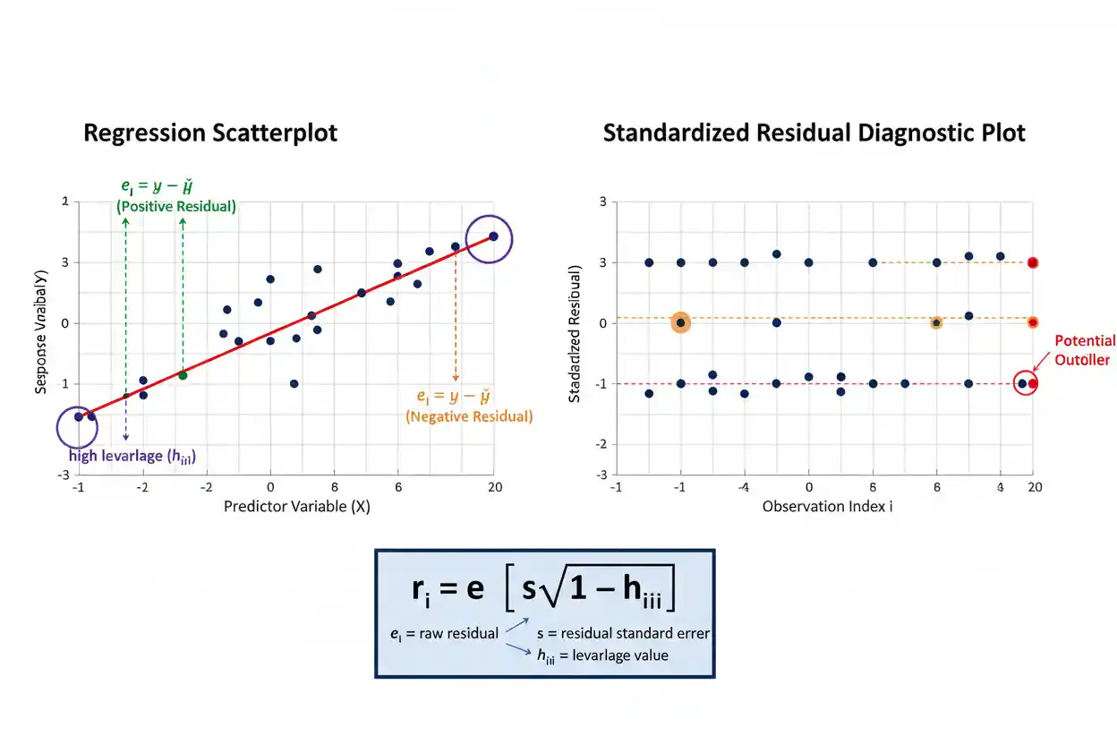
Standardized residuals are regression residuals expressed relative to their estimated standard deviation, allowing prediction errors from different observations to be compared on a common scale. A raw residual tells how many response units an observed value lies above or below its fitted value, but raw residual magnitude alone can be misleading because individual residuals do not necessarily have the same variance. In ordinary least squares regression, observations with different leverage values have different residual variances even when the underlying model assumes constant error variance. A commonly used standardized residual therefore divides the raw residual by the estimated residual standard deviation adjusted by √(1 − hᵢᵢ), where hᵢᵢ is the observation’s leverage.
The resulting value indicates how large the residual is relative to the amount of residual variation expected for that observation. Values near zero indicate observations close to their fitted values, while large positive or negative standardized residuals identify observations whose responses are unusual relative to the fitted regression model. Rules such as ±2 or ±3 are useful diagnostic heuristics, not universal proof that an observation is erroneous or a formal substitute for a prespecified hypothesis test. Standardized residuals are therefore best used as part of a broader regression-diagnostic process that considers residual patterns, leverage, influence, model form, variance assumptions, dependence, and substantive context.
Standardized residuals belong to Statistics & Probability and the broader Inference & Regression framework. Their purpose is narrower than the general study of Residuals: they specifically rescale fitted prediction errors so unusual observations can be evaluated more comparably across a regression dataset.
What Are Standardized Residuals?
Start with an ordinary regression residual:
eᵢ = yᵢ − ŷᵢ
where:
- yᵢ = observed response
- ŷᵢ = fitted response
- eᵢ = raw residual
A raw residual of:
eᵢ = 10
means the observed response lies ten response units above the fitted value.
However, ten units may be very large for one model and completely ordinary for another. Even within the same OLS model, the expected variance of individual residuals can differ because leverage varies across observations.
Standardization divides the residual by an estimate of its own standard deviation.
A common regression diagnostic formula is:
rᵢ = eᵢ / [s√(1 − hᵢᵢ)]
where:
- rᵢ = standardized residual
- eᵢ = raw residual
- s = residual standard error from the fitted model
- hᵢᵢ = leverage of observation i
This transforms residual size into a scale relative to its estimated residual variability.
Standardized Residual Formula
For an ordinary least squares model, the estimated residual variance is based on:
s² = SSE / (n − p)
where:
- SSE = residual sum of squares
- n = number of observations
- p = number of estimated regression parameters, including the intercept
The residual standard error is:
s = √[SSE / (n − p)]
Under the standard homoscedastic linear model, the variance of residual eᵢ conditional on the design matrix is:
Var(eᵢ | X) = σ²(1 − hᵢᵢ)
Replacing the unknown σ with s gives the estimated residual standard deviation:
Estimated SD(eᵢ) = s√(1 − hᵢᵢ)
Therefore:
rᵢ = eᵢ / [s√(1 − hᵢᵢ)]
This leverage adjustment distinguishes the regression-diagnostic standardized residual from the simpler informal calculation eᵢ/s.
Why Raw Residuals Are Not Enough
Suppose two observations both have:
e = 5
It is tempting to say they are equally unusual.
But imagine Observation A has an estimated residual standard deviation of:
1
while Observation B has an estimated residual standard deviation of:
5
Their standardized values would be:
Observation A: 5 / 1 = 5
Observation B: 5 / 5 = 1
The identical five-unit error is extreme for Observation A but ordinary for Observation B relative to its expected residual variability.
Standardization therefore changes the question from:
How many response units did the model miss by?
to:
How large is this miss relative to its expected residual uncertainty?
Both questions are useful, but they answer different diagnostic needs.
Why Leverage Appears in the Formula
In ordinary least squares regression:
ŷ = Hy
where H is the hat matrix.
The diagonal element:
hᵢᵢ
is the leverage of observation i.
Residuals satisfy:
e = (I − H)y
and, under the classical constant-error-variance model:
Var(eᵢ | X) = σ²(1 − hᵢᵢ)
Therefore, residual variance depends on leverage.
Higher leverage means:
hᵢᵢ is larger
so:
1 − hᵢᵢ
is smaller.
This means the raw residual of a high-leverage observation has a smaller model-based variance than that of a typical low-leverage point under the fitted OLS structure.
Dividing by:
√(1 − hᵢᵢ)
adjusts for this difference when residuals are standardized.
What Is Leverage?
Leverage measures how unusual an observation’s predictor values are relative to the predictor configuration represented by the rest of the sample.
In simple regression, observations with x-values far from:
x̄
generally have higher leverage.
With multiple predictors, leverage depends on the observation’s complete predictor combination.
An observation can therefore have individually ordinary predictor values but still possess relatively high leverage if that particular combination of predictor values is unusual.
Leverage is not itself a measure of response error.
An observation can have:
high leverage + tiny residual
or:
low leverage + large residual
These describe different diagnostic properties.
Worked Standardized Residual Example
Suppose a fitted regression predicts:
ŷᵢ = 12
for an observation whose actual response is:
yᵢ = 15
The raw residual is:
eᵢ = yᵢ − ŷᵢ
eᵢ = 15 − 12
eᵢ = 3
Suppose the regression has residual mean square:
MSE = 4
Therefore:
s = √4
s = 2
Suppose the observation has leverage:
hᵢᵢ = 0.36
The standardized residual is:
rᵢ = 3 / [2√(1 − 0.36)]
Continue with:
rᵢ = 3 / [2√0.64]
rᵢ = 3 / [2(0.8)]
rᵢ = 3 / 1.6
rᵢ = 1.875
Therefore:
rᵢ ≈ 1.88
The observation lies approximately 1.88 estimated residual standard deviations above its fitted value.
Why e/s Gives a Different Result
If leverage were ignored, the simpler calculation would be:
eᵢ / s = 3 / 2
= 1.5
But the leverage-adjusted standardized residual is:
1.875
The difference occurs because:
hᵢᵢ = 0.36
reduces the expected variance of that residual under the OLS model.
The full denominator is:
s√(1 − hᵢᵢ)
rather than simply:
s
For regression diagnostics, the leverage-adjusted version usually provides the more informative comparison across observations.
Positive Standardized Residual
A positive standardized residual means:
yᵢ > ŷᵢ
The observed response is above the fitted value.
Suppose:
rᵢ = 2.4
This means the raw residual is positive and approximately 2.4 estimated residual standard deviations above zero according to the chosen standardization.
The sign indicates direction.
The magnitude indicates how unusual the discrepancy is relative to its estimated residual scale.
A positive standardized residual is not automatically evidence that the model systematically underpredicts. One observation may simply lie above its fitted value.
Systematic underprediction would appear as a broader pattern of positive residuals in some region of the predictor space.
Negative Standardized Residual
A negative standardized residual means:
yᵢ < ŷᵢ
Suppose:
rᵢ = −2.7
The observed response lies below the fitted prediction, and its residual magnitude is approximately 2.7 estimated residual standard deviations under the chosen scaling.
A negative sign does not mean the observation is more or less problematic than an equally large positive value.
For many diagnostic purposes:
|rᵢ|
is more relevant to unusualness.
Thus:
rᵢ = +2.7
and:
rᵢ = −2.7
have the same absolute standardized magnitude but opposite prediction-error directions.
Standardized Residual Equal to Zero
If:
eᵢ = 0
then:
rᵢ = 0
provided the denominator is positive.
This occurs when:
yᵢ = ŷᵢ
so the model predicts that observation exactly.
Values close to zero indicate observations lying close to the fitted regression surface relative to their expected residual variability.
A useful model does not require every standardized residual to be near zero. Random variation naturally produces a distribution of positive and negative residuals.
The diagnostic goal is to identify unusual individual values and systematic residual structure rather than demand perfect prediction.
Interpreting Standardized Residual Magnitude
A rough diagnostic interpretation often uses the following ideas:
| Standardized Residual | Typical Diagnostic Interpretation |
|---|---|
| Near 0 | Observation lies close to fitted value |
| Between −2 and +2 | Often not individually remarkable |
| Beyond approximately ±2 | Worth closer examination |
| Beyond approximately ±3 | Potentially unusually extreme |
These are heuristics rather than universal decision rules.
A value of:
2.01
does not suddenly become problematic while:
1.99
is unquestionably normal.
Similarly, a standardized residual above 3 does not prove that an observation is erroneous.
Context, sample size, number of observations examined, leverage, influence, distribution assumptions, and substantive plausibility all matter.
Why ±2 Is Only a Heuristic
If an idealized standardized diagnostic statistic behaved approximately like a standard normal variable, about 95% of values would fall between approximately:
−1.96 and +1.96
for one isolated draw.
This motivates the familiar ±2 heuristic.
But a regression dataset often contains many observations.
If hundreds of residuals are inspected, some values beyond ±2 can occur naturally even when the model is broadly appropriate.
Additionally, internally standardized residuals are not independent standard normal observations. They are generated from the same fitted model and share estimated quantities.
Therefore, ±2 is best treated as a screening guideline rather than as a literal universal hypothesis-test threshold.
Why ±3 Is Often Used for Stronger Screening
Values beyond approximately:
−3 or +3
are less common under light-tailed model behavior and therefore often receive closer scrutiny.
For example:
rᵢ = 3.8
suggests that the response is far from its fitted value relative to the expected residual scale.
However, even a value this large does not answer why it occurred.
Possible explanations include:
- legitimate extreme variation
- data-entry error
- measurement error
- model misspecification
- omitted predictor structure
- heavy-tailed errors
- incorrect variance model
- unusual but valid observation
The diagnostic value flags the observation for investigation; it does not provide the diagnosis itself.
Standardized Residuals vs Raw Residuals
Raw residual:
eᵢ = yᵢ − ŷᵢ
Standardized residual:
rᵢ = eᵢ / estimated SD(eᵢ)
The raw residual preserves the original response units.
If Y is measured in dollars:
eᵢ is measured in dollars
The standardized residual is dimensionless.
This makes raw residuals especially useful for practical error interpretation and standardized residuals especially useful for comparing observations whose expected residual variability differs.
The two should often be examined together.
A standardized value tells how unusual an error is statistically; the raw residual tells how large the error is in real-world units.
Standardized Residuals vs Studentized Residuals
Terminology varies among textbooks and statistical packages.
The leverage-adjusted quantity:
rᵢ = eᵢ / [s√(1 − hᵢᵢ)]
is often called a standardized residual or an internally studentized residual.
Another closely related diagnostic replaces s with an estimate of residual variability calculated after deleting observation i:
tᵢ = eᵢ / [s(i)√(1 − hᵢᵢ)]
where:
s(i)
is the residual standard-error estimate obtained without using observation i in that variance calculation.
This second form is commonly called an externally studentized or deleted residual.
The distinction matters because the suspicious observation contributes to s in the internally standardized version but not to s(i) in the deleted version.
When software reports a column labeled “standardized residual,” its documentation should therefore be checked to determine the exact formula being used.
Why Deleting the Observation Can Matter
Suppose one observation has an exceptionally large residual.
When the full-model residual standard error s is calculated, that large residual contributes to:
SSE
and can inflate s.
The unusually large residual therefore partly increases its own denominator in an internally standardized calculation.
A deleted variance estimate:
s(i)
removes this direct contribution.
For formal outlier assessment, this external studentization can provide useful properties.
For ordinary diagnostic screening, the internally standardized residual remains widely used.
The important point is that “standardized” and “studentized” terminology should not be assumed to mean exactly the same formula in every source.
Standardized Residuals and Residual Plots
A standardized residual plot often displays:
fitted value on the horizontal axis
and:
standardized residual on the vertical axis
A horizontal reference line is drawn at:
0
Additional guides may be drawn at:
+2 and −2
or:
+3 and −3
A suitable linear model with reasonably stable variance should generally produce standardized residuals scattered around zero without systematic structure.
The purpose is not to produce a perfectly random-looking cloud.
Rather, the analyst looks for recurring shapes or unusually extreme values that indicate the regression model may require further examination.
Curved Standardized Residual Pattern
Suppose standardized residuals form a clear U-shaped pattern against fitted values.
Residuals may be:
positive at low fitted values
negative in the middle
positive again at high fitted values
This suggests the fitted conditional mean may be missing nonlinear structure.
A straight-line model could systematically underpredict the ends of the relationship while overpredicting the center.
Standardizing the residuals does not remove the curvature.
It simply puts their magnitudes on a more comparable scale.
The remedy may involve reconsidering the model form rather than deleting individual observations.
Funnel-Shaped Pattern
Suppose standardized residuals appear increasingly dispersed as fitted values increase.
This can indicate that the conditional variability of Y is changing across the predictor range.
However, interpretation requires care because standardizing by the ordinary constant-variance model does not automatically fix heteroscedasticity if the variance model itself is wrong.
A widening pattern may suggest:
Var(ε | X)
is not constant.
Possible responses include modeling the variance structure, transforming the response where scientifically appropriate, or using inference designed to accommodate heteroscedasticity.
The diagnostic pattern identifies a potential variance problem rather than automatically prescribing one specific solution.
Standardized Residuals and Normality
Standardized residuals are often examined with a histogram or normal quantile plot when normal-error assumptions matter for a particular inferential procedure.
A roughly straight pattern in an appropriate normal quantile plot can be consistent with approximate normality.
Strong tail departures, marked skewness, or isolated extreme points can indicate that the assumed error distribution deserves closer examination.
However, fitted residuals are not an independent random sample from the population error distribution.
They are constrained by the regression fit.
Residual normality diagnostics should therefore be interpreted as model checks rather than as proof that the true errors follow an exact normal distribution.
Standardized Residuals and Leverage
A large standardized residual indicates unusual response behavior relative to the fitted model.
High leverage indicates unusual predictor behavior.
These are different dimensions.
Consider Observation A:
standardized residual = 3.2
leverage = low
It has an unusual response but ordinary predictor values.
Observation B might have:
standardized residual = 0.4
leverage = very high
Its response lies close to the fitted line, but its predictor configuration is unusual.
Observation C could have both:
high leverage
and:
large standardized residual
Such observations can be especially influential and deserve careful investigation.
Outlier vs Influential Observation
A response outlier is an observation whose Y value is unusual relative to the fitted model, often reflected by a large standardized or studentized residual.
An influential observation is one whose presence substantially affects fitted results such as regression coefficients or predictions.
These concepts overlap but are not identical.
An observation with a large residual near the center of the predictor distribution can be an outlier without dramatically changing the regression slope.
A high-leverage observation can strongly affect the slope even if its final residual is not exceptionally large.
Standardized residuals therefore contribute one part of influence diagnostics but should not be used alone to decide whether an observation materially controls the fitted model.
Never Remove a Point Only Because |r| Is Large
Suppose:
rᵢ = 3.5
Deleting the observation solely because it exceeds 3 is not a defensible default.
First investigate:
- Was the value entered correctly?
- Was the measurement procedure valid?
- Does the observation belong to the target population?
- Does it reveal a subgroup missing from the model?
- Is the fitted functional form appropriate?
- Does the conclusion change materially when the observation is included?
A valid extreme observation can contain important information about the population.
Removing it simply because it weakens statistical significance or changes a preferred coefficient creates biased analysis.
Standardized Residuals and Sampling Distributions
A Sampling Distribution describes how a statistic such as a sample mean or regression slope varies across repeated samples.
A standardized residual instead concerns one observation’s discrepancy from its fitted value inside one sample.
These concepts operate at different levels.
For a regression slope:
t = (b₁ − β₁,0) / SE(b₁)
standardizes an estimated coefficient relative to its sampling uncertainty.
For an individual regression observation:
rᵢ = eᵢ / [s√(1 − hᵢᵢ)]
standardizes a residual relative to its residual uncertainty.
Both use standardization, but one evaluates an estimator and the other evaluates an observed prediction discrepancy.
Standardized Residuals vs Two-Sample T-Test
A Two-Sample T-Test compares population means from two independent groups under an appropriate t-based framework.
Standardized residuals do not perform that comparison.
For example, a t statistic might compare:
μ₁ − μ₂
with a hypothesized difference.
A standardized residual instead evaluates:
yᵢ − ŷᵢ
for one fitted observation.
Both quantities may be measured in standard-error-like units, but their statistical targets are entirely different.
A large standardized residual is evidence that one observation fits the regression model poorly; it is not evidence that two population means differ.
Standardized Residuals and Significance Level
A Significance Level such as:
α = 0.05
defines the Type I error threshold of a formal hypothesis-testing procedure.
Diagnostic residual cutoffs such as:
|rᵢ| > 2
do not automatically represent α = 0.05 tests.
This distinction becomes especially important when many residuals are inspected.
Suppose a model contains:
n = 500
observations.
Even under relatively well-behaved model conditions, it would not be surprising for some residual diagnostic values to appear moderately extreme simply because hundreds of observations are being examined.
Formal outlier testing requires attention to the relevant statistic, its distribution, and multiplicity rather than mechanically equating ±2 with a significance test.
Multiple Observations and Extreme Residuals
If one approximately standard-normal diagnostic were observed, values beyond ±2 would be relatively uncommon.
But consider hundreds or thousands of observations.
The chance that at least one value appears unusual increases with the number inspected.
This creates a multiple-comparison issue.
Therefore, the largest residual in a dataset should naturally become more extreme as sample size grows, even if the overall model remains appropriate.
A useful diagnostic assessment considers the entire residual distribution rather than applying the same isolated-observation rule without accounting for dataset size.
Standardized Residuals and Statistical Power
Statistical Power concerns the probability that a hypothesis test rejects H₀ when a specified alternative is true.
Standardized residuals do not directly measure statistical power.
However, unusual observations can materially affect residual variance estimates, regression coefficients, and standard errors, which can in turn affect the power and conclusions of regression-based tests.
For example, several extreme residuals may increase:
SSE
and therefore increase:
s
Larger residual variability can reduce coefficient precision, other factors held constant.
Yet removing valid observations simply to increase power would be inappropriate. Power should be improved through sound design, relevant measurements, sufficient independent information, and suitable modeling rather than selective data deletion.
Regression Parameters and Standardized Residuals
The regression model determines fitted values:
ŷᵢ
which determine raw residuals:
eᵢ = yᵢ − ŷᵢ
Those residuals are then standardized.
Changing the model can therefore change every standardized residual.
Suppose an important nonlinear term is omitted. Several observations may initially have large standardized residuals because the linear model systematically misses the relationship.
After an appropriate nonlinear component is added, the same observations may no longer appear unusual.
This does not mean the observations changed.
The model’s representation of expected Y changed.
Residual diagnostics therefore always describe fit relative to a particular model specification.
Effect of Adding Predictors
Adding a relevant predictor can reduce residual variation and change individual fitted values.
Consequently:
eᵢ
may change.
The leverage values:
hᵢᵢ
also change because the predictor design matrix changes.
The residual standard error s can change as well.
Therefore, standardized residuals from two different models should not be assumed to represent the same diagnostic scale even when they are calculated from the same outcome observations.
Each set belongs to its own fitted model.
Model comparison should consider why the specification changed and whether the additional predictors are justified.
Standardized Residuals in Multiple Regression
For multiple regression:
ŷᵢ = b₀ + b₁x₁ᵢ + … + bₖxₖᵢ
the raw residual remains:
eᵢ = yᵢ − ŷᵢ
and the internally standardized residual retains the general form:
rᵢ = eᵢ / [s√(1 − hᵢᵢ)]
The main difference is that leverage now reflects the observation’s complete predictor profile.
An observation can therefore have high leverage because its combination of X₁, X₂, and X₃ is unusual even when none of the predictors individually appears extreme.
This multivariable perspective is one reason standardized residuals and leverage should be examined together.
Average Leverage
In a linear model with:
n observations
and:
p estimated parameters
the leverages satisfy:
Σhᵢᵢ = p
Therefore, average leverage is:
h̄ = p/n
This provides context for determining whether an observation’s leverage is relatively high.
Heuristics such as:
hᵢᵢ > 2p/n
or:
hᵢᵢ > 3p/n
are sometimes used for screening.
Like residual thresholds, these are diagnostic conventions rather than universal laws.
The practical importance of leverage depends on its combination with residual size and actual influence on fitted conclusions.
Why High Leverage Shrinks Raw Residual Variance
At first glance, it may seem strange that:
Var(eᵢ | X) = σ²(1 − hᵢᵢ)
decreases as leverage increases.
A high-leverage point has greater ability to pull the fitted regression surface toward itself.
Because the same observation participates in estimating its own fitted value, its raw residual can become mechanically smaller than the error variance σ² might suggest.
This is precisely why comparing raw residuals without leverage adjustment can understate unusualness for high-leverage observations.
The factor:
√(1 − hᵢᵢ)
compensates for this fitting effect.
Standardized Residuals and Heteroscedasticity
The familiar standardized residual formula assumes the residual variance structure implied by the ordinary homoscedastic model.
If true error variance changes materially across observations, then:
s²(1 − hᵢᵢ)
may not adequately represent each residual’s actual variance.
The resulting standardized residuals can therefore be poorly calibrated in a heteroscedastic model.
This is an important limitation.
Standardization does not automatically repair a misspecified variance model.
If variance systematically changes with predictors or fitted values, the model or diagnostic method should be adapted to that structure.
Standardized Residuals and Dependence
The classical leverage-adjusted formula is developed for the ordinary linear-model dependence structure.
If observations are correlated across time, clusters, subjects, or locations, the covariance matrix of the residuals becomes more complicated.
For example, residuals from repeated measurements on the same person may be correlated.
A value calculated using the ordinary independent-error formula may therefore not have its intended interpretation.
Correct diagnostic standardization should reflect the covariance structure of the model actually fitted.
This is another reason software output should not be interpreted without understanding the underlying model.
Standardized Residuals in Time Series
A regression fitted to time-ordered observations may produce standardized residuals that appear individually moderate but display strong serial patterns.
For example:
+1.1, +1.4, +1.0, +1.3, −1.2, −1.5, −1.1, −1.4
No single value exceeds ±2.
Yet the long runs of same-sign residuals can indicate dependence or an omitted temporal structure.
Therefore, standardized residual magnitude alone is not sufficient.
Residuals should also be examined in their natural order when the data-generating process has temporal structure.
Standardized Residuals and Model Fit
A model with every standardized residual below 2 is not necessarily a good model.
Suppose the residual plot shows a perfect curved wave from:
+1.5 to −1.5
No individual point appears extreme, but the systematic pattern reveals that the fitted mean function is wrong.
Conversely, a well-specified model can occasionally produce one standardized residual slightly above 2 by chance.
Model adequacy therefore depends on:
individual residual magnitude + collective residual pattern
rather than only the maximum absolute value.
Small Standardized Residuals Do Not Prove Good Prediction
A highly flexible model can fit its training observations extremely closely.
This may produce very small residuals and therefore small standardized residuals in the same sample used for estimation.
Yet the model can still perform poorly on new observations if it has captured noise rather than stable structure.
Training residual diagnostics primarily evaluate in-sample fit and model assumptions.
For prediction, out-of-sample validation remains important.
A model that memorizes its training sample is not necessarily a reliable predictive model.
Large Standardized Residuals Do Not Automatically Mean Bad Data
Suppose a legitimate customer spends far more than the model predicts and receives:
rᵢ = 4.1
The observation may be entirely correct.
It could reveal:
- a distinct customer segment
- a missing predictor
- heavy-tailed spending behavior
- a nonlinear relationship
- a rare but real event
Deleting the record would hide information about the population.
Large standardized residuals should prompt investigation, not automatic rejection.
The difference between an invalid observation and a valid extreme observation is substantive, not determined by a numerical cutoff alone.
Standardized Residuals and Data Errors
Standardized residuals can nevertheless be effective tools for detecting potential data problems.
Suppose most model residuals fall between:
−2 and +2
but one observation has:
rᵢ = 12
Further inspection reveals that a response recorded as:
950
should have been:
95
In this case, the diagnostic successfully flagged a data-entry error.
The important step is that the value was corrected because independent evidence established that it was entered incorrectly—not merely because its standardized residual was large.
Diagnostics identify candidates for review; they do not determine the true value.
Standardized Residual Plot Against Predictors
Residuals should sometimes be plotted against individual predictors rather than only against fitted values.
Suppose residuals plotted against X₁ look random but residuals plotted against X₂ show increasing curvature.
This may reveal a misspecified X₂ relationship hidden in the aggregate fitted-value plot.
In multiple regression, examining residuals against:
- predictors
- fitted values
- observation order
- relevant grouping variables
can reveal different model deficiencies.
No single residual plot captures every possible problem.
Diagnostic Reference Lines
A standardized residual plot commonly includes:
r = 0
as the central reference line.
Additional horizontal lines may appear at:
r = +2
r = −2
and sometimes:
r = +3
r = −3
These lines make potentially unusual observations visually easy to locate.
They should be interpreted as guides rather than rigid classification boundaries.
A residual at 2.2 may be less concerning than one at 1.8 if the latter belongs to an influential high-leverage observation or sits within a strong systematic residual pattern.
Diagnostics work best when several pieces of information are considered together.
Worked Comparison of Two Observations
Suppose a regression has:
s = 4
Observation A has:
eA = 6
hAA = 0.10
Its standardized residual is:
rA = 6 / [4√(1 − 0.10)]
= 6 / [4√0.90]
≈ 6 / 3.795
≈ 1.58
Observation B also has:
eB = 6
but:
hBB = 0.75
Then:
rB = 6 / [4√(1 − 0.75)]
= 6 / [4√0.25]
= 6 / 2
= 3
The raw residuals are identical, yet Observation B is substantially more unusual after accounting for its leverage-related residual variance.
This is the central reason regression residual standardization matters.
Why Standardized Residuals Are Dimensionless
The numerator:
eᵢ
has response units.
The denominator:
s√(1 − hᵢᵢ)
also has response units because hᵢᵢ is dimensionless and s uses the units of Y.
Therefore:
response units / response units = dimensionless quantity
This makes standardized residual values more comparable across observations.
However, dimensionless does not mean universally comparable across every unrelated regression model.
Different models may have different error structures, sample sizes, leverage distributions, and assumptions.
The interpretation remains tied to the fitted model that generated the residual.
Common Standardized Residual Mistakes
A common mistake is calculating:
eᵢ/s
and assuming this is always identical to the leverage-adjusted standardized residual. It ignores the factor √(1 − hᵢᵢ).
Another error is treating:
|rᵢ| > 2
as proof that a data point should be deleted.
The value is a diagnostic flag, not a deletion rule.
A third mistake is confusing standardized residuals with standardized regression coefficients or hypothesis-test statistics.
Researchers also sometimes overlook leverage, assuming the largest raw residual must also have the largest standardized residual.
Another error is believing a dataset with no values beyond ±2 automatically satisfies every regression assumption.
Finally, residual thresholds should not be treated as equivalent to a formal Significance Level without an explicitly defined statistical testing procedure.
How to Calculate Standardized Residuals
Begin with the fitted model and calculate each predicted response:
ŷᵢ
Then calculate the raw residual:
eᵢ = yᵢ − ŷᵢ
Calculate the model residual standard error:
s = √[SSE/(n − p)]
Obtain the leverage:
hᵢᵢ
for each observation.
Then calculate:
rᵢ = eᵢ / [s√(1 − hᵢᵢ)]
Repeat this for every observation.
The resulting standardized residuals can then be plotted against fitted values, predictors, observation order, or other relevant diagnostic dimensions.
Investigate both large individual magnitudes and systematic collective patterns.
How to Interpret Standardized Residuals
Suppose:
rᵢ = 0.3
The observation lies relatively close to its fitted value.
Suppose:
rᵢ = −1.7
The response is below its prediction but not exceptionally far away according to common diagnostic heuristics.
Suppose:
rᵢ = 3.4
The observation is unusually far above its fitted response relative to its estimated residual variability and deserves closer inspection.
The correct next question is not:
Should I delete it?
Instead ask:
Why does this observation disagree so strongly with the model?
That question leads to meaningful diagnostic analysis.
How to Report Standardized Residual Diagnostics
A useful regression report should summarize relevant residual behavior rather than list every standardized residual.
For example:
Standardized residuals were generally centered around zero without a strong systematic pattern; most fell between −2 and +2, while one observation exceeded +3 and was examined for data quality and influence.
If the unusual observation is valid, say so.
If the residual plot shows curvature or changing spread, report the pattern rather than implying that individual outlier screening alone established model adequacy.
Diagnostic reporting should connect residual evidence to the consequences for model interpretation, inference, or prediction.
Frequently Asked Questions
What are standardized residuals?
Standardized residuals are raw regression residuals divided by an estimate of their standard deviation so prediction errors can be compared on a common scale.
What is the formula for a standardized residual?
A common OLS regression formula is:
rᵢ = eᵢ / [s√(1 − hᵢᵢ)]
What is eᵢ?
The raw residual:
eᵢ = yᵢ − ŷᵢ
What is s?
s is the regression residual standard error:
s = √[SSE/(n − p)]
What is hᵢᵢ?
hᵢᵢ is the leverage of observation i, obtained from the diagonal of the regression hat matrix.
Why is leverage included?
Under the classical OLS model:
Var(eᵢ | X) = σ²(1 − hᵢᵢ)
so observations with different leverage values have different raw residual variances.
What does a positive standardized residual mean?
The observed response is above the fitted prediction.
What does a negative standardized residual mean?
The observed response is below the fitted prediction.
What does a standardized residual of zero mean?
The observation is predicted exactly:
yᵢ = ŷᵢ
Is a standardized residual above 2 an outlier?
It can be a useful diagnostic flag, but ±2 is a heuristic rather than a universal proof of outlier status.
What does a standardized residual above 3 mean?
It indicates an unusually large prediction discrepancy under common diagnostic conventions and generally deserves investigation, but it does not prove the value is incorrect.
Should observations above ±3 be removed?
No. Investigate data quality, model specification, leverage, influence, and substantive validity before considering any exclusion.
What is the difference between residuals and standardized residuals?
Raw residuals are measured in the response’s original units. Standardized residuals divide those errors by an estimate of their residual standard deviation and are dimensionless.
Is eᵢ/s always the standardized residual?
Not necessarily. In regression diagnostics, a leverage-adjusted form using √(1 − hᵢᵢ) is commonly used.
What is the difference between standardized and studentized residuals?
Terminology varies. The internally studentized quantity commonly uses the full-model residual standard error s, while an externally studentized residual uses a variance estimate calculated with the observation deleted.
Are standardized residuals normally distributed?
They can exhibit approximately normal-like behavior under suitable model conditions, but internally standardized residuals are not simply independent standard normal observations. Their exact behavior depends on the fitted model.
Why plot standardized residuals against fitted values?
The plot can reveal curvature, changing variance, unusual observations, and other evidence of model misspecification.
What does a U-shaped residual pattern mean?
It can indicate missing nonlinear structure in the fitted mean relationship.
What does a funnel-shaped pattern mean?
It can indicate changing residual variance, or heteroscedasticity.
Are standardized residuals the same as z-scores?
They share the general idea of scaling a deviation by a standard-deviation-like quantity, but the regression formula accounts for fitted-model residual variability and leverage.
Are standardized residuals the same as t statistics?
No. A coefficient t statistic standardizes an estimated parameter relative to its sampling uncertainty. A standardized residual scales an individual prediction discrepancy.
Do standardized residuals measure leverage?
No. Leverage describes predictor unusualness. Standardized residuals describe response discrepancy relative to the fitted model, although leverage appears in their scaling.
Can a point have high leverage and a small standardized residual?
Yes. Its predictor profile can be unusual while its observed response lies close to the fitted model.
Can a large standardized residual have low leverage?
Yes. An observation with ordinary predictor values can have an unusually large response discrepancy.
Do standardized residuals determine statistical power?
No. Statistical power concerns the probability of rejecting a null hypothesis under a specified alternative. Residual variation can affect coefficient precision and therefore power, but standardized residuals themselves are diagnostic quantities.
Key Takeaway
Standardized residuals place regression prediction errors on a common diagnostic scale. The raw residual is:
eᵢ = yᵢ − ŷᵢ
and a common leverage-adjusted standardized residual is:
rᵢ = eᵢ / [s√(1 − hᵢᵢ)]
where s is the residual standard error and hᵢᵢ is the observation’s leverage.
This adjustment matters because OLS residuals do not all have the same variance:
Var(eᵢ | X) = σ²(1 − hᵢᵢ)
under the standard homoscedastic regression model. Two observations with identical raw residuals can therefore have substantially different standardized residuals if their leverage values differ.
Values near zero indicate observations close to their fitted responses. Values beyond approximately ±2 are often examined more closely, and values beyond approximately ±3 can indicate unusually large discrepancies. These numbers are diagnostic heuristics rather than automatic rejection rules or universal hypothesis-test thresholds.
Most importantly, standardized residuals should be interpreted as one part of model diagnostics. Large values can arise from valid extreme observations, data problems, missing predictors, incorrect functional form, heavy tails, changing variance, or other model deficiencies. Their usefulness comes not from mechanically deleting observations but from identifying where the fitted model and the observed data disagree enough to warrant careful investigation.



