Statistical power is the probability that a hypothesis-testing procedure correctly rejects the null hypothesis when a specified alternative condition is true. It measures a study’s ability to detect an effect of a particular size rather than the probability that an observed result is correct. If β represents the probability of a Type II error—failing to reject the null hypothesis under a specified alternative—then statistical power is 1 − β. A power of 0.80 means that, if the assumed effect and all other design conditions used in the calculation were repeatedly reproduced, the testing procedure would reject the null hypothesis approximately 80% of the time.
Power depends on several factors, including effect size, sample size, variability, the chosen Significance Level, whether the test is one-sided or two-sided, allocation between groups, measurement precision, and the statistical procedure itself. Larger samples and larger true effects generally increase power, while greater unexplained variability reduces it. Lowering α usually decreases power when everything else remains fixed because stronger evidence is then required for rejection. Power calculations are therefore most useful before data collection, when they can help determine how much information is needed to detect an effect that would actually matter.
Statistical power is a fundamental concept in Statistics & Probability and Inference & Regression. It is defined through the behavior of a test statistic’s Sampling Distribution under alternatives to the null hypothesis and should always be interpreted relative to a specific effect size and testing procedure.
What Is Statistical Power?
Suppose a hypothesis test evaluates:
H₀: θ = θ₀
against an alternative:
H₁: θ ≠ θ₀
The test has a rejection region determined by the chosen significance level.
If H₀ is actually false and the true parameter is some specified alternative value:
θ = θ₁
the test may either correctly reject H₀ or fail to reject it.
The probability of correctly rejecting H₀ at θ₁ is the power:
Power(θ₁) = P(reject H₀ | θ = θ₁)
If β denotes the probability of failing to reject H₀ under that same alternative:
β = P(fail to reject H₀ | θ = θ₁)
then:
Power = 1 − β
Power is therefore the complement of the Type II error probability for a specified alternative.
Statistical Power Formula
The basic formula is:
Power = 1 − β
where:
- Power = probability of detecting the specified alternative
- β = probability of a Type II error
The deeper definition is:
Power(θ) = Pθ(test statistic falls in rejection region)
This notation makes an important point: power is usually a function of the true parameter value.
There is not necessarily one universal power number for a study.
A test might have:
Power = 0.25
for a tiny effect,
Power = 0.80
for a moderate effect,
and:
Power = 0.99
for a large effect.
The probability of detection changes because different true effects shift the alternative sampling distribution by different amounts.
Type I Error vs Type II Error
The two principal errors in classical hypothesis testing are:
Type I Error
Rejecting H₀ when H₀ is true.
Its probability is controlled by:
α
For a simple null hypothesis:
α = P(reject H₀ | H₀ true)
Type II Error
Failing to reject H₀ when a specified alternative is true.
Its probability is:
β
Therefore:
Statistical power = 1 − β
The two error probabilities are related through the design of the test, but they are not generally equal.
A procedure with:
α = 0.05
does not automatically have:
β = 0.05
or:
Power = 0.95
Power must be calculated separately for a specified alternative.
What Does 80% Power Mean?
Suppose a planned experiment has:
Power = 0.80
for detecting a population mean difference of 5 units.
This means that if the true effect really is 5 units and the complete study design is repeatedly replicated under the assumptions used in the calculation, approximately 80% of those studies would reject H₀ using the specified testing rule.
The remaining:
20%
would fail to reject H₀ despite the assumed five-unit effect.
That 20% is:
β = 0.20
because:
1 − 0.20 = 0.80
It does not mean there is an 80% probability that a particular significant result is true.
It also does not mean there is an 80% probability that the assumed effect exists.
Statistical Power Depends on the Alternative
Consider:
H₀: μ = 100
Suppose a study has good power when the true mean is:
μ = 110
but much poorer power when the true mean is:
μ = 101
This is expected.
A ten-unit departure from H₀ shifts the alternative sampling distribution much farther from the null distribution than a one-unit departure.
The test therefore has a greater probability of crossing its rejection threshold under the larger effect.
Power should consequently be stated with the effect used to calculate it.
Saying only:
“The study has 80% power”
is incomplete unless the targeted alternative is clear.
The Power Function
A power function expresses power across possible parameter values:
π(θ) = Pθ(reject H₀)
Under the null value in a properly calibrated simple test:
π(θ₀) = α
As θ moves farther into alternatives that the test is designed to detect, power generally increases.
For a two-sided test, power typically rises as the true parameter moves sufficiently far either above or below the null value.
A graphical power curve therefore often has its lowest value around the null and rises as the effect becomes more extreme.
This provides a more complete view than reporting power for only one assumed effect.
Why Sampling Distributions Determine Power
Power can be understood by comparing two Sampling Distribution scenarios.
First consider the distribution of a test statistic when H₀ is true. The significance level determines a critical boundary in this null distribution.
Now consider the distribution when a specific alternative is true.
The same critical boundary remains in place, but the alternative distribution is shifted.
The proportion of the alternative distribution lying inside the rejection region is:
Power
The proportion remaining outside the rejection region is:
β
Thus power is literally an area under an alternative sampling distribution.
Null and Alternative Distributions
Imagine a right-tailed z-test.
Under H₀:
Z-like statistic is centered according to the null condition
and the upper α portion defines the rejection region.
Suppose the true parameter is larger than the null value. The statistic’s distribution shifts to the right.
The farther it shifts, the more probability lies beyond the critical boundary.
Therefore:
larger true effect → larger power
The relationship is not mysterious. Power increases because the alternative distribution becomes more separated from the null distribution relative to its sampling spread.
Five Major Factors That Affect Statistical Power
Statistical power is especially influenced by:
- effect size
- sample size
- variability
- significance level
- testing design and direction
These factors interact.
For example, a small effect can still be detected with high power if the sample is sufficiently large and measurements are precise.
A large effect can remain difficult to detect in a tiny sample with extreme variability.
Power calculations therefore evaluate the complete combination rather than any one factor in isolation.
Effect Size and Statistical Power
Effect size measures how far the true population condition is from the null condition.
Suppose:
H₀: μ₁ − μ₂ = 0
If the true difference is:
0.1
the alternative distribution may overlap heavily with the null distribution.
If the true difference is:
10
the distributions may be much more separated.
All else equal:
larger effect size → greater statistical power
This is why power should be calculated for an effect that is substantively meaningful rather than simply any nonzero effect.
Detecting a scientifically trivial difference with high probability may not make a study useful.
Standardized Effect Size
For a difference in means, a standardized effect can take the form:
d = Δ / σ
where:
- Δ = population mean difference of interest
- σ = relevant population standard deviation
Suppose:
Δ = 5
and:
σ = 10
Then:
d = 5/10
d = 0.5
A standardized effect expresses the targeted difference in standard-deviation units.
This is useful in power calculations because doubling the difference has the same standardized effect as halving the standard deviation, other conditions held equal.
Sample Size and Statistical Power
Increasing sample size generally increases power because standard errors decrease.
For a mean:
SE(x̄) = σ/√n
As n grows:
SE decreases
A fixed population effect therefore becomes larger relative to its sampling uncertainty.
Suppose the true difference from H₀ is:
Δ = 4
If:
SE = 4
the standardized signal is:
4/4 = 1
If a larger sample reduces the standard error to:
SE = 1
then:
4/1 = 4
The same underlying effect is now much easier for the test to distinguish from the null condition.
Why Sample Size Has Diminishing Returns
Because standard error usually decreases with:
√n
sample size must grow substantially to achieve progressively smaller standard errors.
For example, suppose:
SE ∝ 1/√n
To cut the standard error in half, sample size must be multiplied by approximately:
4
To reduce it to one-third, sample size must be multiplied by approximately:
9
This square-root relationship means that increasing a study from 100 to 200 observations helps, but it does not halve the standard error.
Larger samples improve power, but the gain is not linear.
Variability and Statistical Power
Higher variability makes effects harder to distinguish from background noise.
Suppose two studies target the same mean difference:
Δ = 5
Study A has:
σ = 5
Study B has:
σ = 25
The standardized effects are:
Study A: d = 5/5 = 1
Study B: d = 5/25 = 0.2
The first effect is large relative to ordinary observation-level variation, while the second is comparatively small.
With equivalent sample sizes and testing procedures, Study A will generally have greater statistical power.
Reducing measurement noise can therefore improve power without increasing sample size.
Significance Level and Statistical Power
The Significance Level determines how extreme a test statistic must be before H₀ is rejected.
Suppose a right-tailed standard normal test uses:
α = 0.05
The critical value is approximately:
1.645
If α is reduced to:
0.01
the critical value moves to approximately:
2.326
The alternative distribution must now extend farther into the tail before the test rejects H₀.
Therefore, holding effect size and sample size fixed:
smaller α → lower Type I error probability
but usually:
smaller α → lower power
This is the fundamental tradeoff between stricter false-positive control and sensitivity to true alternatives.
Increasing Alpha Increases Power
If α is increased, the rejection region becomes larger.
For example, changing a right-tailed test from:
α = 0.01
to:
α = 0.05
moves the critical boundary closer to the null center.
A larger proportion of the alternative distribution then lies in the rejection region.
Power increases.
However, this also increases the probability of rejecting H₀ when H₀ is actually true.
Choosing α merely to make a study more powerful is therefore not a free improvement. It changes the test’s false-positive operating characteristics.
One-Sided vs Two-Sided Tests
A one-sided test places the entire α probability into one tail.
A two-sided test divides α between two tails.
At:
α = 0.05
a right-sided standard normal test has approximate critical value:
1.645
while a two-sided test has upper critical boundary:
1.96
For a genuinely positive alternative, the one-sided test therefore has greater power because the rejection boundary is closer.
However, it sacrifices the ability to reject for sufficiently strong effects in the opposite direction.
One-sided testing should be chosen because the research question genuinely excludes the opposite direction from the inferential claim, not because the observed data happen to favor one side.
Two-Sample Tests and Power
When comparing two independent population means, power depends on:
- targeted mean difference
- group variances
- sample sizes
- allocation ratio
- significance level
- test direction
- chosen testing procedure
A Two-Sample T-Test commonly estimates variance from the sample, while a classical Two-Sample Z-Test uses known population standard deviations or another setting supporting z-based inference.
The same conceptual power framework applies to both:
specify an alternative difference
determine the sampling distribution under that alternative
calculate the probability that the test statistic crosses the rejection threshold
Approximate Sample Size Formula for Two Means
For two independent groups of equal size, equal population standard deviation σ, a two-sided z-based comparison, significance level α, desired power 1 − β, and targeted difference Δ, an approximate sample size per group is:
n ≈ 2σ²(z₁₋α/₂ + z₁₋β)² / Δ²
Using standardized effect:
d = Δ/σ
this becomes:
n ≈ 2(z₁₋α/₂ + z₁₋β)² / d²
This formula is useful for understanding how sample size changes with α, desired power, and effect size.
Exact calculations for particular tests may differ, especially when variance is estimated or assumptions are more complex.
Worked Power and Sample Size Example
Suppose researchers plan a two-group comparison and want:
α = 0.05
for a two-sided test,
Power = 0.80
and a targeted standardized difference:
d = 0.50
The relevant normal quantiles are approximately:
z₁₋α/₂ = z₀.975 ≈ 1.96
and:
z₁₋β = z₀.80 ≈ 0.842
Using:
n ≈ 2(1.96 + 0.842)² / 0.50²
First:
1.96 + 0.842 = 2.802
Square it:
2.802² ≈ 7.851
Multiply by 2:
2 × 7.851 ≈ 15.702
Divide by:
0.50² = 0.25
Therefore:
n ≈ 15.702 / 0.25
n ≈ 62.81
Round upward:
n ≈ 63 participants per group
The approximate total sample is therefore:
126 participants
under the assumptions of this simplified z-based design.
Why Sample Size Is Rounded Up
Suppose a power calculation produces:
n = 62.2
participants per group.
Using 62 would fall below the calculated requirement.
Therefore, the usual approach is:
round upward to 63
not downward.
Additional allowance may also be required for:
- anticipated missing observations
- participant withdrawal
- unusable measurements
- design effects
- clustering
The analytical power requirement should generally refer to the usable sample rather than merely the number initially recruited.
Effect of a Smaller Target Difference
Use the same design but target:
d = 0.25
instead of:
d = 0.50
The sample-size relationship contains:
1/d²
Halving d therefore multiplies the required sample size by approximately:
4
The previous requirement was about:
63 per group
so the smaller effect requires approximately:
252 per group
under the same simplified assumptions.
Small effects require much larger samples because their alternative distributions lie closer to the null.
Effect of Higher Desired Power
Suppose researchers increase desired power from:
0.80
to:
0.90
Then:
z₀.80 ≈ 0.842
becomes:
z₀.90 ≈ 1.282
The sample-size formula therefore increases because:
z₁₋β
is larger.
Higher desired power means the test must detect the specified effect more consistently across repeated studies.
That requires more information unless some other design feature improves, such as lower measurement variance.
80% Power Is a Convention, Not a Universal Requirement
A target such as:
80% power
is common but not universally optimal.
In some high-stakes settings, missing a meaningful effect may be costly enough to justify:
90%
or even higher planned power.
In exploratory work, resource constraints may lead to different decisions.
The chosen target should reflect:
- consequences of false negatives
- consequences of false positives
- minimum meaningful effect
- feasibility
- study cost
- ethical considerations
Like α = 0.05, power = 0.80 is a convention that should be justified rather than treated as a law.
Minimum Detectable Effect
Power calculations can be rearranged to answer a different question:
Given my sample size, what effect can this design detect with a specified probability?
This quantity is often called the minimum detectable effect.
Suppose n is fixed because only a limited population is available.
Rather than asking:
“How many observations do I need?”
the analyst can ask:
“With the observations available, how large must the true effect be for this test to have 80% power?”
This perspective is often more informative than merely reporting that the study is “powered.”
It connects the design directly with the smallest effect it can reliably detect.
Power and Unequal Group Sizes
For equal-variance two-group comparisons with similar cost per observation, equal allocation generally provides good or optimal efficiency:
n₁ ≈ n₂
Suppose a total of 100 participants is available.
A:
50/50
split generally provides more information about the difference than an extreme:
90/10
split under otherwise symmetric conditions.
Unequal allocation can still be justified when:
- one group is more expensive
- exposure availability differs
- variances differ
- ethical constraints apply
- recruitment capacity differs
But imbalance can reduce power for a fixed total sample.
Power and Paired Designs
Pairing or repeated measurement can increase power when observations within each pair are positively correlated.
For paired measurements:
D = X − Y
and:
Var(D) = Var(X) + Var(Y) − 2Cov(X,Y)
If:
Cov(X,Y) > 0
the variance of the differences can be substantially smaller than the variance that would arise from treating observations as unrelated.
A smaller variance of D means a smaller standard error of the mean difference and potentially greater power.
However, pairing only helps when the paired structure is genuine and appropriately modeled.
Artificially pairing unrelated observations does not create valid precision.
Measurement Reliability and Power
Poor measurement can reduce statistical power.
Suppose a true outcome varies meaningfully with treatment, but the measurement instrument adds substantial random noise.
That noise increases observed variability.
The effect becomes smaller relative to the standard error, making it harder for the test to distinguish the alternative from H₀.
Improving measurement reliability can therefore increase power without recruiting additional observations.
Good study design is not simply about sample size. Precise instruments, consistent procedures, and high-quality measurements can materially improve inferential efficiency.
Restricted Predictor or Exposure Variation
Power can also decrease when the variable representing the relevant exposure or predictor has little variation.
Suppose a study seeks to estimate how an outcome changes across a continuous exposure, but nearly everyone has almost the same exposure value.
There is little information about differences across the predictor.
Even a large nominal sample may provide limited power for detecting the relationship.
Study design should therefore consider where observations lie, not only how many observations exist.
More rows do not always mean proportionally more information.
Clustering and Effective Sample Size
Suppose a study collects 1,000 observations from only ten highly homogeneous clusters.
Observations within each cluster may be strongly correlated.
The dataset contains:
n = 1,000 rows
but substantially less than 1,000 independent pieces of information.
Ignoring clustering can produce an overly optimistic power calculation because the assumed sampling variance is too small.
Clustered designs require power methods that incorporate quantities such as:
- number of clusters
- average cluster size
- intracluster correlation
- allocation across clusters
Adding more observations within the same highly correlated clusters may provide less benefit than adding new independent clusters.
Missing Data and Achieved Information
Suppose a planned study requires:
200 complete observations
for its target power.
If researchers recruit exactly 200 participants but only:
160
provide usable outcomes, the effective power may be lower than planned.
A design may therefore inflate recruitment to account for anticipated attrition.
For example, if 20% loss is expected, a rough recruitment target to obtain 200 complete observations is:
200 / (1 − 0.20)
= 200 / 0.80
= 250
This calculation assumes the missing-data process itself does not introduce additional bias or complexity.
More recruitment cannot repair systematic missingness automatically.
Multiple Testing Can Reduce Power
Suppose many hypotheses are tested while familywise Type I error is controlled.
A procedure may require each individual test to use a more stringent effective significance threshold.
For example, a simple Bonferroni strategy for ten tests with familywise:
α = 0.05
uses:
αindividual = 0.005
A smaller individual α moves the rejection threshold farther into the tail.
That reduces power for each specific test unless sample size or effect magnitude increases.
Multiplicity planning should therefore occur before data collection when many confirmatory comparisons are expected.
Power and Standardized Residuals
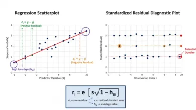
Standardized Residuals are diagnostic quantities rather than measures of power, but regression residual behavior can affect the assumptions and variance estimates underlying a power calculation.
Large unexplained residual variability tends to produce larger standard errors.
That can reduce the probability that a genuine coefficient or group difference crosses its testing threshold.
Extreme residual patterns can also suggest:
- heteroscedasticity
- nonlinear structure
- omitted variables
- unusual observations
- incorrect model assumptions
If the model assumed for the power calculation poorly reflects the actual data-generating process, the achieved operating characteristics can differ substantially from those planned.
Power and Statistical Significance
A study can have high planned power but still produce a nonsignificant result.
If:
Power = 0.80
for a specified effect,
then even when that exact effect is true:
β = 0.20
so approximately 20% of repeated studies would still fail to reject H₀ under the assumed design.
Likewise, a low-powered study can occasionally produce a significant result.
Power is a repeated-sampling property of a testing procedure under specified alternatives, not a guarantee of the result obtained in one particular sample.
High Power Does Not Guarantee a True Result
Imagine a study with:
Power = 0.95
for a specified effect.
If the null hypothesis is actually true, power against that alternative is not what determines the false-positive probability.
The relevant quantity is:
α
A highly powered test can still make Type I errors at its configured significance level.
Power and false-positive control answer different conditional questions:
α = P(reject H₀ | H₀ true)
Power = P(reject H₀ | specified alternative true)
Neither is the probability that the hypothesis is true after observing the result.
Low Power Does Not Make Significant Results Automatically False
A low-powered study is less likely to detect the targeted effect when it exists.
However, if it obtains a statistically significant result, one cannot conclude from low power alone that the finding is false.
Low power can contribute to unstable estimates, wide confidence intervals, and selective-significance problems across a research process, but evaluating one result requires considering:
- design
- effect estimate
- uncertainty
- assumptions
- multiplicity
- prior evidence
- potential bias
Power should not be converted into a posterior probability of truth or falsehood.
Nonsignificant Result in a Low-Power Study
Suppose a study has only:
Power = 0.30
for an effect considered scientifically meaningful.
The result is:
p = 0.25
The correct conclusion is not:
“There is no meaningful effect.”
The study was unlikely to detect that effect even if it existed.
A nonsignificant result from a low-power design can therefore be highly inconclusive.
The confidence interval may remain compatible with both no effect and important effects.
Power considerations help explain why failure to reject H₀ does not establish equivalence or absence of an effect.
High Power and Nonsignificant Results
Suppose a study has high power to detect effects larger than a prespecified meaningful threshold and still produces a precise estimate close to zero.
That combination can provide stronger evidence that large effects are unlikely.
However, this conclusion is better expressed through the actual effect estimate and confidence interval than through “observed power.”
If the interval excludes effects considered practically important, the data directly demonstrate that those effect sizes are inconsistent with the estimate at the interval’s confidence level.
Power planning and interval estimation complement one another but answer different questions.
Why Post-Hoc Observed Power Is Often Misleading
After a study has been completed, some analysts insert the observed effect estimate into a power formula and calculate “observed power.”
For many standard hypothesis tests, this quantity is largely a transformation of the observed test statistic or p-value.
If the result is nonsignificant, observed power will usually be low.
If the result is highly significant, observed power will usually be high.
This does not add much independent information about the result and can encourage circular reasoning.
After data collection, effect estimates and confidence intervals generally provide more direct information about magnitude and precision.
Power is most valuable when used prospectively for design.
Prospective vs Retrospective Power
Prospective power is calculated before data are observed using:
- targeted effect size
- planned sample size
- assumed variability
- α
- test structure
Its purpose is to design an informative study.
Retrospective power based on the observed effect often tells little beyond what is already encoded in the observed significance result.
A completed study should therefore generally be interpreted using:
estimated effect + confidence interval + test result + design quality
rather than claiming that a nonsignificant outcome is explained simply because “observed power was low.”
Power Is Not the Probability the Alternative Is True
Suppose:
Power = 0.90
This means:
P(reject H₀ | specified alternative true) = 0.90
It does not mean:
P(alternative true | data) = 0.90
These conditional probabilities are reversed.
Likewise, if a study fails to reject H₀, one cannot say:
“There is a 10% chance the alternative is true because power was 90%.”
Power is a characteristic of the procedure under an assumed parameter value, not a probability assigned to competing hypotheses after observing data.
Statistical Power vs Confidence Level
Confidence level and power are also different.
A 95% confidence interval corresponds in many standard two-sided procedures to:
α = 0.05
The confidence level is related to Type I error control.
Power concerns Type II error under a specified alternative:
Power = 1 − β
A study can use:
95% confidence intervals
while having:
30%, 80%, or 99% power
depending on sample size, effect size, and variability.
Confidence level alone does not determine power.
Power and Practical Significance
Suppose a huge study has nearly 100% power to detect an effect of:
d = 0.05
Such an effect may still be practically negligible.
The purpose of power analysis should therefore not be:
detect any nonzero effect
but rather:
reliably detect an effect large enough to matter
A minimum meaningful difference should ideally be defined using subject-matter considerations before the sample size calculation.
Otherwise, a very large dataset can be designed to detect differences that have little practical value.
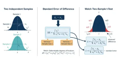
Power and Two-Sample T-Tests
A Two-Sample T-Test generally has power determined by the separation between population means relative to their standard error.
For equal-sized groups with similar variability, greater n reduces uncertainty in the estimated mean difference.
The t distribution also reflects uncertainty from estimating variance.
As sample sizes grow, the relevant t critical values approach their normal counterparts.
Therefore, z-based formulas are often useful for approximate planning, while exact or software-based t-test power calculations can incorporate finite-sample details more accurately.
The underlying logic remains:
effect signal / sampling noise
determines how far the alternative test-statistic distribution moves from the null distribution.
Power and Two-Sample Z-Tests
A Two-Sample Z-Test provides a particularly transparent setting for power because the relevant standard-normal distributions can often be written explicitly under known-variance assumptions.
For an estimated difference:
x̄₁ − x̄₂
with known population variances:
SE = √(σ₁²/n₁ + σ₂²/n₂)
A larger true difference increases the standardized shift:
Δ / SE
while larger samples reduce SE.
Both effects increase separation between the null and alternative distributions and therefore increase power.
Common Statistical Power Mistakes
A common mistake is saying:
“Power of 80% means the hypothesis has an 80% chance of being detected as true.”
Power is conditional on an assumed alternative; it does not assign truth probabilities to hypotheses.
Another mistake is reporting one power number without specifying the effect size for which it was calculated.
A third error is assuming a nonsignificant result from a highly underpowered study proves no effect.
Researchers also sometimes calculate post-hoc power using the observed effect and treat the resulting number as new evidence.
Another mistake is increasing α solely to make a study more powerful without recognizing that Type I error also increases.
Finally, sample size should not be inflated mechanically without considering bias, dependence, measurement quality, and whether the targeted effect is actually meaningful.
How to Calculate Statistical Power
A general power calculation follows several steps.
First, state the null and alternative hypotheses.
Second, specify:
α
Third, define the effect size under the alternative.
Fourth, determine the sampling distribution of the test statistic under that alternative.
Fifth, identify the rejection region using the null distribution.
Finally, calculate:
Power = P(test statistic falls in rejection region | specified alternative)
For simple textbook tests this can be calculated analytically.
For more complicated models, power may require numerical integration or simulation.
The conceptual definition remains identical.
How to Plan a Study Using Power
A practical planning sequence is:
Define the smallest effect that would be important enough to detect.
Choose an appropriate significance level.
Select the statistical test that matches the design.
Estimate realistic variability from prior evidence, pilot information, or justified assumptions.
Choose the desired power.
Calculate the required usable sample size.
Then adjust recruitment for expected loss, clustering, unequal allocation, or other design features.
The effect assumption deserves particular scrutiny because an unrealistically large assumed effect can produce a sample-size requirement that is far too small.
Sensitivity Analysis for Power
Because power calculations depend on uncertain assumptions, it is often useful to calculate several scenarios.
For example:
| Scenario | Standardized Effect | Desired Power | Approximate Requirement |
|---|---|---|---|
| Larger effect | 0.60 | 0.80 | Lower sample |
| Moderate effect | 0.40 | 0.80 | Higher sample |
| Smaller effect | 0.25 | 0.80 | Much higher sample |
| Moderate effect, stronger power | 0.40 | 0.90 | Higher than 80% target |
This reveals how sensitive the design is to assumptions.
A study whose feasibility depends entirely on an optimistic effect estimate may be fragile.
Sensitivity analysis is often more informative than reporting one seemingly exact sample-size number.
How to Report Statistical Power
A useful power statement should identify the assumptions that produced the number.
Instead of saying:
“Power was 80%.”
a more informative statement is:
“The planned design targeted 80% power for detecting a standardized two-group mean difference of d = 0.50 using a two-sided α = 0.05 test.”
If sample size was calculated from assumed variance in original units, state that assumption as well.
The report should make clear whether the power calculation was prospective or based on the observed result.
For completed studies, confidence intervals and effect estimates should remain central to interpretation.
Frequently Asked Questions
What is statistical power?
Statistical power is the probability that a hypothesis-testing procedure rejects H₀ when a specified alternative condition is true.
What is the statistical power formula?
Power = 1 − β
where β is the Type II error probability for the specified alternative.
What is a Type II error?
A Type II error occurs when a test fails to reject H₀ even though the specified alternative is true.
What does 80% power mean?
It means the procedure would reject H₀ approximately 80% of the time under repeated studies when the particular alternative used in the calculation is true and the assumptions hold.
Does 80% power mean an 80% chance the alternative hypothesis is true?
No. Power is conditional on the alternative being true; it does not provide a probability that the alternative is true.
Does power depend on effect size?
Yes. Larger true effects are usually easier to distinguish from H₀ and therefore have higher power.
Does sample size affect power?
Yes. Larger samples usually reduce standard errors and increase power.
Does variability affect power?
Yes. Greater unexplained variability generally reduces power because the effect becomes harder to distinguish from background noise.
Does alpha affect power?
Yes. Increasing α generally increases power but also increases the Type I error probability. Decreasing α generally reduces power when everything else is fixed.
Does a one-sided test have more power?
For an effect in the prespecified direction, a one-sided test generally has more power at the same total α because the entire rejection probability is allocated to one tail.
Should I choose a one-sided test just to increase power?
No. The direction should be justified by the research question before examining the data.
Is 80% power always enough?
No. It is a common convention, but the appropriate target depends on the costs of false negatives, study purpose, feasibility, and consequences of decisions.
What is 90% power?
It corresponds to:
β = 0.10
for the specified alternative.
Can a high-powered study produce a nonsignificant result?
Yes. Power below 1 means some repeated studies will fail to reject H₀ even when the targeted alternative is true.
Can a low-powered study produce a significant result?
Yes. Low power means significance is less likely under the specified alternative, not impossible.
Does low power prove a significant result is false?
No.
Does a nonsignificant result prove no effect?
No, especially when the study has poor ability to detect effects of practical importance.
What is minimum detectable effect?
It is an effect magnitude that a design can detect with a specified level of power at a chosen α.
Why do smaller effects need larger samples?
Small effects produce alternative sampling distributions closer to the null distribution. More observations are needed to reduce standard error and distinguish them reliably.
Why does quadrupling sample size roughly halve standard error?
Because standard error often follows:
SE ∝ 1/√n
Can better measurement increase power?
Yes. Reducing measurement noise can reduce variability and improve the ability to detect a genuine effect.
Does clustering affect power?
Yes. Correlated observations provide less independent information than the same number of independent observations, so clustered designs need specialized power calculations.
Is observed post-hoc power useful after a study?
Power computed from the observed effect is often largely determined by the observed test statistic and adds little beyond the p-value. Effect estimates and confidence intervals are usually more informative after data collection.
How is power related to significance level?
Alpha controls false-positive probability under H₀, while power controls detection probability under a specified alternative:
α = P(reject H₀ | H₀ true)
Power = P(reject H₀ | specified alternative true)
Is statistical power the same as practical importance?
No. A study can have enormous power to detect an effect too small to matter in practice.
Key Takeaway
Statistical power measures a test’s ability to detect a specified departure from the null hypothesis:
Power = P(reject H₀ | specified alternative true)
and:
Power = 1 − β
where β is the probability of a Type II error.
Power is not a fixed property of a study independent of effect size. It changes according to the alternative being considered. Larger effects, larger samples, lower variability, more efficient study designs, and less restrictive rejection thresholds generally increase power. Lowering the significance level provides stronger Type I error control but usually reduces power unless additional information is collected.
For an approximate equal-sized two-group z-based design, sample size illustrates these relationships directly:
n ≈ 2σ²(z₁₋α/₂ + z₁₋β)² / Δ²
or using standardized effect d:
n ≈ 2(z₁₋α/₂ + z₁₋β)² / d²
The squared effect in the denominator explains why detecting increasingly small differences can require dramatically larger samples.
Most importantly, power is best used prospectively. A meaningful design identifies the smallest effect worth detecting, chooses an appropriate Type I error threshold, estimates realistic variability, and then determines how much independent information is required. After data have been collected, the observed effect and its confidence interval generally provide more direct information than a post-hoc power calculation. Statistical power is therefore not a probability that a hypothesis is true; it is a repeated-sampling property describing how reliably a specified testing procedure can detect a specified effect.