
A two-sample t-test is an inferential statistical procedure used to compare the means of two independent populations when population standard deviations are not treated as known. The test asks whether the observed difference between two sample means is large relative to the sampling variability expected under a specified null hypothesis, most commonly that the population means are equal. Two major forms are used: Welch’s two-sample t-test, which does not assume equal population variances, and the pooled two-sample t-test, which uses a common-variance assumption. Welch’s procedure is generally the more flexible default for independent groups because it allows the sample variances and sample sizes to differ, while the pooled version is appropriate when the equal-variance model is substantively justified.
The test statistic standardizes the difference between sample means by an estimated standard error, producing a t value that can be compared with an appropriate Student’s t reference distribution. A small p-value can provide evidence against the null mean difference, but it does not measure the probability that the null hypothesis is true, the size of the effect, or the practical importance of the difference. Correct use also requires genuinely independent groups, an outcome for which comparing means is meaningful, and a sampling structure capable of supporting the intended inference.
The two-sample t-test belongs to Statistics & Probability and the broader Inference & Regression framework. Its central purpose is to compare two independent population means while accounting for uncertainty from estimating the groups’ variability.
What Is a Two-Sample T-Test?
Suppose two independent populations have means:
μ₁
and:
μ₂
A researcher collects one sample from each population and calculates:
x̄₁
and:
x̄₂
The observed difference is:
x̄₁ − x̄₂
The most common null hypothesis is:
H₀: μ₁ − μ₂ = 0
which is equivalent to:
H₀: μ₁ = μ₂
A two-sided alternative is:
H₁: μ₁ − μ₂ ≠ 0
The test asks whether the observed sample difference is unusually large relative to the amount of sample-to-sample variation expected if the null model were correct.
The core structure is:
t = (observed difference − hypothesized difference) / estimated standard error
For two independent sample means:
t = [(x̄₁ − x̄₂) − Δ₀] / SE(x̄₁ − x̄₂)
where:
Δ₀
is the population mean difference specified by H₀.
Usually:
Δ₀ = 0
but the method can test other hypothesized differences.
Welch Two-Sample T-Test Formula
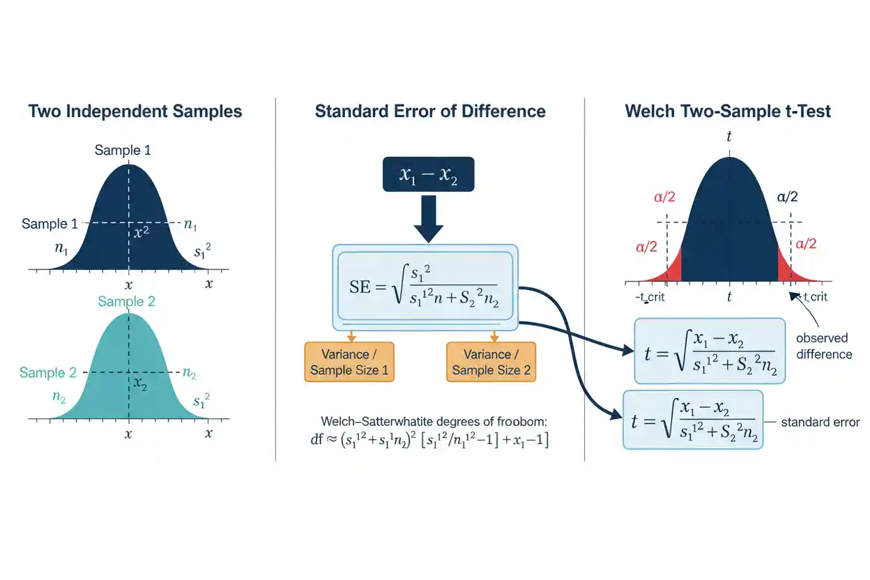
For two independent samples with no equal-population-variance assumption, Welch’s t statistic is:
t = [(x̄₁ − x̄₂) − Δ₀] / √(s₁²/n₁ + s₂²/n₂)
where:
- x̄₁ = mean of Sample 1
- x̄₂ = mean of Sample 2
- s₁² = sample variance of Group 1
- s₂² = sample variance of Group 2
- n₁ = Group 1 sample size
- n₂ = Group 2 sample size
- Δ₀ = hypothesized population mean difference
For the common null:
H₀: μ₁ − μ₂ = 0
the formula simplifies to:
t = (x̄₁ − x̄₂) / √(s₁²/n₁ + s₂²/n₂)
The denominator is the estimated standard error of the difference between independent sample means.
Welch Degrees of Freedom
Welch’s test uses approximate degrees of freedom:
df ≈ (s₁²/n₁ + s₂²/n₂)² / {[(s₁²/n₁)²/(n₁−1)] + [(s₂²/n₂)²/(n₂−1)]}
This expression is known as the Welch–Satterthwaite approximation.
The resulting df does not need to be an integer.
For example:
df ≈ 19.93
is mathematically valid.
Statistical software can evaluate the t distribution using fractional degrees of freedom directly.
The adjustment reflects uncertainty created by estimating two potentially different population variances.
Pooled Two-Sample T-Test Formula
The pooled form assumes:
σ₁² = σ₂² = σ²
That common population variance is estimated by combining the two sample variances.
The pooled variance is:
sₚ² = [(n₁−1)s₁² + (n₂−1)s₂²] / (n₁+n₂−2)
The pooled standard deviation is:
sₚ = √sₚ²
The standard error of the mean difference becomes:
SE = sₚ√(1/n₁ + 1/n₂)
and the pooled t statistic is:
t = [(x̄₁ − x̄₂) − Δ₀] / [sₚ√(1/n₁ + 1/n₂)]
The degrees of freedom are:
df = n₁ + n₂ − 2
This procedure is valid when the common-variance model is appropriate. It should not be selected merely because an equal-variance preliminary test failed to reject.
Welch vs Pooled T-Test
The central distinction is the treatment of population variances.
Welch’s test permits:
σ₁² ≠ σ₂²
The pooled test assumes:
σ₁² = σ₂²
Welch’s procedure separately incorporates:
s₁²/n₁
and:
s₂²/n₂
into the standard error.
The pooled procedure first combines the variance estimates into:
sₚ²
and then applies the same pooled variance to both groups.
When population variances are genuinely equal, both methods often produce similar results, especially when sample sizes are similar. When variances differ—particularly together with unequal group sizes—the pooled test can have poorly calibrated uncertainty, whereas Welch’s method is specifically constructed to accommodate unequal variances.
For that reason, Welch’s two-sample t-test is often a sensible general-purpose choice for independent mean comparisons.
Worked Two-Sample T-Test Example
Suppose two independent training programs are compared using a quantitative performance score.
Group 1 has:
n₁ = 12
x̄₁ = 74
s₁ = 8
Group 2 has:
n₂ = 10
x̄₂ = 66
s₂ = 7
The research question is whether the population mean performance differs between the two programs.
Use:
H₀: μ₁ − μ₂ = 0
and:
H₁: μ₁ − μ₂ ≠ 0
The observed difference is:
x̄₁ − x̄₂ = 74 − 66
= 8
Group 1’s sample mean is eight points higher than Group 2’s.
Step 1: Calculate Each Variance
For Group 1:
s₁² = 8²
s₁² = 64
For Group 2:
s₂² = 7²
s₂² = 49
Step 2: Calculate the Standard Error
For Welch’s test:
SE = √(s₁²/n₁ + s₂²/n₂)
Substitute:
SE = √(64/12 + 49/10)
Calculate each component:
64/12 ≈ 5.333
49/10 = 4.900
Therefore:
SE = √(5.333 + 4.900)
SE = √10.233
SE ≈ 3.199
The estimated standard error of the sample mean difference is approximately:
3.20 points
Step 3: Calculate the T Statistic
The null difference is:
Δ₀ = 0
Therefore:
t = (8 − 0) / 3.199
t ≈ 2.50
The observed difference is about 2.5 estimated standard errors above the zero-difference null.
Step 4: Calculate Welch Degrees of Freedom
Use:
df ≈ (5.333 + 4.900)² / [(5.333²/11) + (4.900²/9)]
The numerator is:
10.233² ≈ 104.72
The denominator is approximately:
28.44/11 + 24.01/9
≈ 2.59 + 2.67
≈ 5.26
Therefore:
df ≈ 104.72 / 5.26
df ≈ 19.9
So the test result is approximately:
t(19.9) = 2.50
Step 5: Find the P-Value
For a two-sided test with:
t ≈ 2.50
and:
df ≈ 19.9
the p-value is approximately:
p ≈ 0.021
If the chosen Significance Level is:
α = 0.05
then:
p < α
so the null hypothesis is rejected.
The sample provides statistical evidence that the two population means differ under the assumptions of the Welch two-sample t-test.
This does not mean the probability that H₀ is true is 2.1%. It also does not determine whether an eight-point difference is practically important.
Confidence Interval for the Mean Difference
A Welch confidence interval has the form:
(x̄₁ − x̄₂) ± t* × SE
For the worked example:
x̄₁ − x̄₂ = 8
SE ≈ 3.199
df ≈ 19.9
A 95% t critical value is approximately:
t* ≈ 2.09
The margin of error is therefore about:
2.09 × 3.199
≈ 6.69
The approximate confidence interval is:
8 ± 6.69
giving:
Lower limit ≈ 1.31
Upper limit ≈ 14.69
Therefore:
95% CI ≈ 1.3 to 14.7 points
The interval excludes zero, which is consistent with rejection of the corresponding two-sided zero-difference hypothesis at α = 0.05.
How to Interpret the Confidence Interval
The estimated population mean difference is eight points.
The confidence interval indicates substantial uncertainty around that estimate:
approximately 1.3 to 14.7 points
A frequentist 95% confidence interval does not mean there is a 95% posterior probability that the fixed population difference now lies inside that particular realized interval.
Its interpretation concerns the long-run coverage of the interval-generating procedure under its assumptions.
The interval is especially useful because it shows magnitude and precision rather than merely whether the null value crosses a significance threshold.
Independent Samples Are Essential
The standard two-sample t-test is designed for two independent samples.
Examples include:
Group A participants vs different Group B participants
Treatment group vs separately assigned control group
customers from Region A vs different customers from Region B
The observations in one group should not be natural counterparts of observations in the other group under the standard independent-samples framework.
If the same individuals are measured twice or units are deliberately matched into pairs, the dependence should be modeled rather than ignored.
Using an independent two-sample test on strongly paired observations can produce an inappropriate standard error because the procedure discards the within-pair covariance structure.
Independence Within Groups
Independence is also relevant within each sample.
Suppose 100 measurements are obtained from only five individuals, with 20 repeated measurements from each person.
Those 100 values should not automatically be treated as 100 independent observations.
Measurements from the same person may be correlated.
Similarly, students within the same classroom, patients within the same clinic, or observations within the same household can share common influences.
A standard two-sample t-test that ignores such clustering can substantially understate uncertainty.
The correct sampling unit and dependence structure must therefore be identified before calculating the test.
Quantitative Outcome
A two-sample t-test compares means, so the response variable should be quantitative and measured on a scale for which arithmetic means and differences are meaningful.
Examples can include:
- height
- response time
- temperature
- test score
- production amount
- blood pressure
A categorical outcome such as:
success/failure
is not naturally analyzed through a standard comparison of arithmetic means unless represented within a suitable statistical framework where that coding and inference are justified.
The inferential procedure should match the type of outcome rather than being selected solely because two groups are present.
Normality and the Two-Sample T-Test
The exact classical t distribution is derived under assumptions about normal population errors or observations within the relevant model.
Welch’s t-test can still perform well under moderate non-normality, particularly when sample sizes provide enough stable information and severe outliers or extreme skewness are absent.
However, there is no universal sample size that guarantees robustness.
A small sample drawn from a strongly skewed or heavy-tailed population can produce unreliable mean-based t inference.
The relevant issue is not simply whether a histogram looks perfectly bell-shaped but whether the sampling distribution of the mean difference and standard-error estimate behave adequately for the intended inference.
No Universal n = 30 Rule
A common shortcut suggests that each group merely needs:
n ≥ 30
for the t-test to become valid.
That is not a universal statistical rule.
For approximately normal populations without serious outliers, much smaller samples can support exact or strong t-based inference.
For highly skewed or heavy-tailed populations, 30 observations per group may still provide inadequate approximation.
Validity depends on:
- distribution shape
- tail behavior
- outliers
- independence
- sample-size balance
- variance structure
- inferential objective
Sample size should therefore be assessed with the data-generating context rather than one rigid threshold.
Outliers and Mean Comparisons
The sample mean and sample standard deviation are both sensitive to extreme observations.
Suppose Group 1 consists mostly of scores between:
60 and 80
but contains one value of:
500
That observation can strongly alter:
x̄₁
and:
s₁
The effect on the t statistic can be complicated because it changes both the estimated difference and its standard error.
An unusual observation should be investigated for data quality and substantive validity.
A legitimate extreme value should not be deleted simply because its removal creates a smaller p-value or a preferred conclusion.
Unequal Variances
Suppose:
s₁ = 5
and:
s₂ = 25
The sample variances differ dramatically.
Welch’s test directly allows the two variance estimates to contribute separately:
SE = √(s₁²/n₁ + s₂²/n₂)
The pooled test instead assumes both samples estimate the same underlying σ².
If that assumption is seriously wrong, especially with unequal sample sizes, pooled standard errors can become misleading.
Welch’s test avoids requiring the equal-variance assumption and is therefore particularly useful when group variability differs.
Why Unequal Sample Sizes Matter With Unequal Variances
The combination of unequal variances and unequal sample sizes can be especially important for pooled inference.
Suppose the smaller group has much larger variance.
A pooled common-variance estimate can distribute the variance information in a way that poorly represents the actual uncertainty of the mean difference.
Welch’s standard error preserves:
s₁²/n₁
and:
s₂²/n₂
separately, then adjusts degrees of freedom accordingly.
This makes the test better suited to heteroscedastic two-group comparisons.
Equal sample sizes can make some variance inequality less damaging for pooled methods, but they do not make the equal-variance assumption literally true.
Should You Test Equal Variances First?
A common workflow performs a preliminary variance-equality test and then chooses between pooled and Welch t-tests depending on its p-value.
This approach can be problematic.
Failing to reject equal variances does not prove that the population variances are equal, particularly with small samples.
The two-stage decision also changes the behavior of the overall procedure.
If equal population variances are not substantively required by the scientific model, directly using Welch’s test avoids making the mean comparison depend on a preliminary hypothesis test.
The pooled procedure is most defensible when a common variance is part of the intended model rather than merely a consequence of failing to detect variance inequality.
Equal-Variance Pooled Example
Using the worked data:
n₁ = 12, s₁² = 64
n₂ = 10, s₂² = 49
the pooled variance is:
sₚ² = [(12−1)(64) + (10−1)(49)] / (12+10−2)
sₚ² = [11(64) + 9(49)] / 20
sₚ² = (704 + 441) / 20
sₚ² = 1145 / 20
sₚ² = 57.25
Therefore:
sₚ = √57.25
sₚ ≈ 7.57
The pooled standard error is:
SE = 7.57√(1/12 + 1/10)
which is approximately:
3.23
This is close to Welch’s 3.20 because the sample variances and sizes in this example are not dramatically different.
In other datasets, the discrepancy can be much larger.
Two-Sample T-Test vs Two-Sample Z-Test
The Two-Sample Z-Test and two-sample t-test share the same fundamental goal of standardizing a difference between independent sample estimates.
The major distinction in the classical mean-comparison setting concerns how population variability is handled.
A z procedure can use known population standard deviations:
σ₁ and σ₂
giving:
z = [(x̄₁−x̄₂)−Δ₀] / √(σ₁²/n₁ + σ₂²/n₂)
The two-sample t-test instead uses estimated standard deviations:
s₁ and s₂
and accounts for variance-estimation uncertainty through a t reference distribution and appropriate degrees of freedom.
Large sample size alone does not magically make unknown population standard deviations known.
T Distribution vs Normal Distribution
Student’s t distributions are symmetric and centered at zero like the standard normal distribution, but they have heavier tails.
The amount of extra tail weight depends on degrees of freedom.
With low df, the t distribution has noticeably heavier tails.
As:
df → ∞
the t distribution approaches:
Normal(0,1)
This reflects the fact that estimating variance from a small sample introduces additional uncertainty.
As sample information grows, the variance estimate becomes more stable and the distinction between t and normal reference distributions decreases.
One-Sided Two-Sample T-Test
Suppose Group 1 is expected to have a larger population mean than Group 2.
A directional hypothesis could be:
H₀: μ₁ − μ₂ ≤ 0
H₁: μ₁ − μ₂ > 0
The rejection region lies in the upper tail.
A sufficiently large positive t statistic supports rejection.
If the observed statistic is strongly negative, it does not support this right-tailed alternative.
The direction of a one-sided test should be specified from the research question before examining the data.
Choosing a one-sided test after observing which sample mean is larger invalidates the intended directional error-rate interpretation.
Left-Tailed Test
If the research question predicts:
μ₁ < μ₂
the hypotheses may be:
H₀: μ₁ − μ₂ ≥ 0
H₁: μ₁ − μ₂ < 0
The rejection region lies in the lower tail.
A large negative t statistic provides evidence in the specified direction.
The sign of:
x̄₁ − x̄₂
therefore matters for one-sided testing.
Reversing the group order reverses the sign of both the estimated difference and t statistic but does not change the corresponding two-sided p-value.
Two-Sided Test
The common two-sided hypotheses are:
H₀: μ₁ − μ₂ = 0
H₁: μ₁ − μ₂ ≠ 0
Both sufficiently positive and sufficiently negative differences provide evidence against H₀.
The two-sided p-value includes extremeness in both directions according to the t reference distribution.
A two-sided procedure is generally appropriate when meaningful departures could occur in either direction.
It should not be converted to a one-sided procedure after observing the sign of the result merely to reduce the reported p-value.
Testing a Nonzero Difference
The null hypothesis need not be zero.
Suppose two manufacturing processes are considered comparable around a benchmark difference of:
Δ₀ = 2
A test can evaluate:
H₀: μ₁ − μ₂ = 2
using:
t = [(x̄₁−x̄₂)−2] / SE
If the observed difference is:
8
the numerator becomes:
8 − 2 = 6
The test now asks whether the population difference departs from two, not whether the population means are equal.
This illustrates why the null difference should always be explicitly stated.
Difference in Means vs Difference in Individual Observations
Suppose a test estimates:
μ₁ − μ₂ = 8
This concerns the difference between population means.
It does not mean every observation in Group 1 is eight units larger than every observation in Group 2.
The group distributions can overlap substantially.
For example, both populations may have standard deviations around:
20
while their means differ by eight.
Many individuals in the lower-mean group can therefore score above individuals in the higher-mean group.
A two-sample t-test compares averages, not perfect separation between populations.
Statistical Significance vs Effect Size
Suppose a study estimates:
x̄₁ − x̄₂ = 0.2
with:
SE = 0.02
Then:
t = 10
and the p-value will be extremely small.
Yet a difference of 0.2 units may be practically negligible.
Another study might estimate:
x̄₁ − x̄₂ = 10
with:
SE = 8
giving:
t = 1.25
The second sample shows a much larger numerical difference but much greater uncertainty.
Statistical significance therefore reflects effect magnitude relative to uncertainty, not effect magnitude alone.
Standardized Effect Size
One way to complement the raw mean difference is with a standardized effect size.
Under an equal-variance framework, a Cohen-style standardized difference can be written:
d = (x̄₁ − x̄₂) / sₚ
Using the worked example:
x̄₁ − x̄₂ = 8
and:
sₚ ≈ 7.57
Therefore:
d ≈ 8 / 7.57
d ≈ 1.06
This expresses the observed mean difference in pooled standard-deviation units.
The standardized effect should not replace the raw difference when the original units are meaningful.
Different standardized-effect definitions may also be preferred under unequal variances or small-sample correction frameworks, so the denominator and method should be stated clearly.
Statistical Power
Statistical Power is the probability that the two-sample test rejects H₀ when a specified alternative difference is true.
Power generally increases with:
- larger population mean differences
- larger independent sample sizes
- smaller within-group variability
- more efficient allocation
- a less stringent α
For a fixed total sample under similar variances and observation costs, reasonably balanced group sizes often provide good precision.
A study should ideally be planned around the smallest mean difference that would matter in practice rather than around an arbitrary goal of detecting any nonzero difference.
Sample Size and Precision
For Welch’s mean difference:
SE = √(s₁²/n₁ + s₂²/n₂)
Increasing either sample size reduces its corresponding variance contribution.
Suppose:
s₁² = s₂² = 100
and initially:
n₁ = n₂ = 25
Then:
SE = √(100/25 + 100/25)
= √8
≈ 2.83
If both samples increase to:
n₁ = n₂ = 100
then:
SE = √(100/100 + 100/100)
= √2
≈ 1.41
Quadrupling both group sizes approximately halves the standard error.
Balanced vs Unbalanced Samples
When group variances and observation costs are similar, balanced samples:
n₁ ≈ n₂
often provide efficient estimation of the mean difference.
Suppose a total sample of:
100
can be divided as:
50 and 50
or:
90 and 10
Under equal variances, the standard-error component:
1/n₁ + 1/n₂
is much smaller for the balanced allocation.
The 90/10 design therefore provides less precision for the difference despite having the same total number of observations.
Unequal allocation can still be justified by cost, ethics, availability, or unequal variances, but its effect on precision should be considered.
Missing Data
A standard independent two-sample t-test uses the observations available in each group under the chosen analysis.
If missing outcomes are related to treatment response, group membership, or outcome severity, simply analyzing complete observations can introduce bias.
Increasing the original recruitment total does not automatically solve this problem.
Missing-data handling should be considered as part of the study design and inferential model.
The validity of a t-test depends not only on the arithmetic sample sizes but also on whether the analyzed observations represent the intended populations appropriately.
Random Assignment vs Random Sampling
Random assignment and random sampling solve different inferential problems.
Random assignment helps support causal comparisons between treatment conditions by balancing potential confounders in expectation.
Random sampling helps support generalization from the sample to a broader population.
A two-sample t-test itself does not create either property.
If participants self-select into two groups, the t-test can quantify the mean difference and its sampling uncertainty under the model but does not automatically establish that group membership caused that difference.
Study design determines the scope of the conclusion.
Two-Sample T-Test Does Not Prove Causation
Suppose Group 1 has an average income eight units higher than Group 2 and:
p < 0.01
This is statistical evidence of a population mean difference under the testing model.
It does not establish why the difference exists.
Potential explanations could include:
- group-defining exposure
- age differences
- education
- geography
- selection
- measurement differences
- other confounding factors
A randomized experiment can support stronger causal interpretation than an observational comparison, but even randomized studies require attention to compliance, attrition, measurement, and implementation.
The t-test provides inference about means; causal interpretation comes from design and assumptions.
Two-Sample T-Test vs Two-Way ANOVA
A Two-Way Anova addresses a broader factorial structure involving two categorical explanatory factors and can evaluate main effects and interactions.
A two-sample t-test instead focuses on a single comparison between two independent population means.
For example:
Treatment A vs Treatment B
with one grouping variable and two levels is naturally a two-sample mean-comparison problem.
A design involving:
Treatment A/B × Male/Female
contains two factors and potentially an interaction, requiring a broader model if those effects are part of the research question.
Using repeated separate t-tests cannot reproduce the complete factorial inference provided by a properly specified two-way ANOVA.
Multiple Comparisons
A two-sample t-test handles one defined mean comparison.
Suppose five groups are present and every pair is compared using separate unadjusted tests at:
α = 0.05
The probability of obtaining at least one false rejection across the family can become much larger than 5%.
A multi-group or multiple-comparison framework may therefore be more appropriate.
This is one reason the two-sample t-test should remain scoped to a genuine two-group comparison rather than being repeatedly applied to every pair in a larger factorial dataset without considering multiplicity.
Relationship to Linear Regression
A two-group comparison can also be expressed as a linear regression using a binary indicator.
Let:
G = 0 for Group 2
G = 1 for Group 1
Fit:
Y = β₀ + β₁G + ε
Then:
β₀ = mean of Group 2
and:
β₁ = μ₁ − μ₂
Under the corresponding variance assumptions, testing:
H₀: β₁ = 0
is equivalent to testing equality of the two population means.
This connection illustrates that the two-sample t-test is part of the broader linear-model framework rather than an isolated statistical technique.
Welch T-Test and Heteroscedastic Regression
Welch’s test can also be viewed in relation to regression with a two-level indicator and unequal group variances.
The essential idea is to estimate the group mean difference while allowing uncertainty to reflect separate group variance estimates.
This distinguishes it from the pooled common-variance model.
The regression perspective becomes especially useful when additional covariates or more complex design features need to be incorporated.
The basic two-sample t-test, however, owns the direct unadjusted comparison of two independent means.
Standardized Residuals and Two-Sample Models
Standardized Residuals are diagnostic quantities that evaluate individual observations relative to fitted predictions.
They are not substitutes for the two-sample test statistic.
In a regression representation of a two-group comparison, residual diagnostics can reveal:
- unusual observations
- variance differences
- heavy tails
- other departures from the fitted model
A large standardized residual may identify one observation that fits the group model poorly.
The two-sample t statistic instead evaluates the difference between the two group means relative to its standard error.
These quantities operate at different levels of analysis.
Significance Level and the Decision Rule
Suppose the chosen Significance Level is:
α = 0.05
The p-value rule is:
p ≤ 0.05 → reject H₀
p > 0.05 → fail to reject H₀
This threshold should generally be defined before seeing the result.
A result such as:
p = 0.049
should not be treated as fundamentally different evidence from:
p = 0.051
merely because the conventional threshold lies between them.
The actual effect estimate and confidence interval provide essential context around the binary testing decision.
Failure to Reject H₀
Suppose:
p = 0.30
The correct conclusion is ordinarily:
fail to reject H₀
not:
prove that μ₁ = μ₂
A nonsignificant result can arise because:
- the true difference is zero or small
- the samples are too small
- variability is high
- the estimate is imprecise
- assumptions are poorly matched
- the study has low power
If the objective is to demonstrate that two population means are sufficiently similar within a predefined practical margin, an equivalence procedure is needed rather than interpreting a nonsignificant ordinary t-test as proof of equality.
Example of an Imprecise Nonsignificant Difference
Suppose:
x̄₁ − x̄₂ = 8
but the 95% confidence interval is:
−10 to 26
The interval contains zero, so a corresponding two-sided test would fail to reject equality at α = 0.05.
But the interval also includes substantial positive differences and moderate negative differences.
The data are therefore compatible with many possibilities.
Saying:
“There is no difference”
would overstate the evidence.
The more accurate conclusion is that the study estimates the group difference too imprecisely to determine its direction and magnitude confidently.
Very Large Samples
Suppose millions of independent observations are available.
A difference of:
0.01
can produce an extremely small p-value if the standard error becomes sufficiently tiny.
This demonstrates that:
statistically detectable ≠ practically important
A large study can estimate tiny population differences very precisely.
The two-sample t-test answers whether the difference is distinguishable from the specified null under the model.
Whether the difference matters requires substantive judgment and usually benefits from examining the confidence interval and effect magnitude.
Very Small Samples
A two-sample t-test can be used with small samples under suitable model assumptions, particularly when group distributions are reasonably compatible with the relevant normal model.
However, small samples provide limited information for diagnosing:
- skewness
- extreme tails
- variance differences
- influential observations
They also produce less precise estimates and heavier-tailed t reference distributions.
A significant result can still occur in a small study, but conclusions should account for the resulting uncertainty.
Small n does not automatically invalidate a t-test, just as large n does not automatically validate every model assumption.
Pooled Degrees of Freedom
For the equal-variance pooled t-test:
df = n₁ + n₂ − 2
Why subtract two?
The two group means consume two pieces of information when the common variance is estimated from within-group deviations.
The pooled variance numerator contains:
(n₁−1)s₁² + (n₂−1)s₂²
with total degrees of freedom:
(n₁−1) + (n₂−1)
= n₁ + n₂ − 2
Welch’s method cannot use this simple df because it retains separate variance estimates rather than assuming one common population variance.
Relationship Between T and Confidence Interval
For a two-sided test of:
H₀: μ₁ − μ₂ = Δ₀
the null value and a compatible confidence interval provide equivalent decision information.
If the corresponding 95% confidence interval excludes:
Δ₀
the two-sided α = 0.05 test rejects that null value.
If the interval includes Δ₀, the corresponding test fails to reject it.
However, the interval provides additional information because it shows a range of plausible parameter values under the procedure rather than only a reject/fail-to-reject decision.
Common Two-Sample T-Test Mistakes
A common mistake is using the independent two-sample t-test for paired or repeated observations. Dependence should be modeled rather than ignored.
Another error is assuming equal sample sizes imply equal population variances. They do not.
Researchers also sometimes select the pooled test simply because a preliminary variance test is nonsignificant. Failing to detect variance inequality does not establish equality.
Another frequent mistake is interpreting:
p > 0.05
as proof that the population means are equal.
It is also incorrect to interpret a small p-value as the probability H₀ is true or as proof that group membership caused the outcome difference.
Finally, focusing entirely on the p-value while omitting the raw mean difference and confidence interval conceals the magnitude and precision of the result.
How to Calculate a Two-Sample T-Test
For Welch’s two-sample t-test, begin with:
x̄₁, x̄₂, s₁, s₂, n₁, n₂
State the hypotheses:
H₀: μ₁ − μ₂ = Δ₀
H₁: μ₁ − μ₂ ≠ Δ₀
Calculate the observed difference:
x̄₁ − x̄₂
Then calculate:
SE = √(s₁²/n₁ + s₂²/n₂)
Next:
t = [(x̄₁−x̄₂)−Δ₀] / SE
Calculate the Welch–Satterthwaite degrees of freedom:
df ≈ (s₁²/n₁ + s₂²/n₂)² / {[(s₁²/n₁)²/(n₁−1)] + [(s₂²/n₂)²/(n₂−1)]}
Use the t reference distribution to obtain the p-value or critical-value decision.
Finally, calculate and interpret a confidence interval for:
μ₁ − μ₂
and evaluate the assumptions, design, and practical importance of the estimated difference.
How to Report a Two-Sample T-Test
A useful report should include the sample means, estimated difference, t statistic, degrees of freedom, p-value, and confidence interval.
For the worked example:
Group 1 mean = 74
Group 2 mean = 66
Mean difference = 8 points
t(19.9) ≈ 2.50
p ≈ 0.021
95% CI ≈ 1.3 to 14.7 points
A contextual report could state that Group 1’s mean was estimated to be eight points higher than Group 2’s, with the confidence interval indicating that the population difference is plausibly positive but still estimated with substantial uncertainty.
The practical importance of that range should then be interpreted using the actual measurement scale.
Frequently Asked Questions
What is a two-sample t-test?
A two-sample t-test compares the means of two independent populations using sample data when population standard deviations are estimated rather than treated as known.
What is the Welch two-sample t-test formula?
t = [(x̄₁−x̄₂)−Δ₀] / √(s₁²/n₁ + s₂²/n₂)
What is usually tested?
The most common null is:
H₀: μ₁ − μ₂ = 0
What does Δ₀ mean?
Δ₀ is the population mean difference specified by the null hypothesis.
What is the difference between Welch and pooled t-tests?
Welch’s test allows unequal population variances. The pooled test assumes a common population variance.
Which two-sample t-test should I use?
Welch’s test is generally useful when equal population variances are not substantively assumed. A pooled test is appropriate when a common-variance model is justified.
Does Welch’s test require equal sample sizes?
No.
Does Welch’s test require equal variances?
No.
Can Welch degrees of freedom be decimal?
Yes. Fractional degrees of freedom such as 19.9 are valid.
What is the pooled variance formula?
sₚ² = [(n₁−1)s₁² + (n₂−1)s₂²] / (n₁+n₂−2)
What are pooled-test degrees of freedom?
df = n₁ + n₂ − 2
What is the difference between a two-sample t-test and two-sample z-test?
A classical z-test uses known population standard deviations or another justified z framework. The t-test estimates variability from sample data and uses a t reference distribution.
Must the groups be independent?
Yes for the standard two-sample t-test. Paired or matched observations require a method that accounts for their dependence.
Does equal sample size mean the groups are independent?
No. Independence is determined by the sampling or study structure, not by sample counts.
Does equal sample size mean equal variance?
No.
Does the outcome have to be normal?
Exact classical small-sample inference relies on normal population assumptions, while t procedures can be reasonably robust to moderate non-normality under suitable conditions. Severe skewness, heavy tails, or outliers require more care.
Is n = 30 always enough?
No. There is no universal n = 30 guarantee.
What does a positive t statistic mean?
When the difference is defined as x̄₁ − x̄₂, a positive t statistic indicates the observed difference is above the null difference.
Does a significant t-test mean every person in Group 1 scores higher?
No. The test concerns population means, and the individual group distributions can overlap considerably.
Does p < 0.05 prove the means are meaningfully different?
No. It addresses statistical evidence relative to the null. Practical importance depends on the size and context of the difference.
Does p > 0.05 prove equal means?
No. Failure to reject equality does not establish equivalence.
Does a significant two-sample t-test prove causation?
No. Causal interpretation depends on the study design and assumptions.
Why should I report a confidence interval?
It communicates both the estimated difference and its uncertainty rather than reducing the analysis to a threshold decision.
What affects statistical power for the two-sample t-test?
Effect size, sample sizes, group variability, allocation, significance level, test direction, and design quality all affect power.
Key Takeaway
The two-sample t-test evaluates a difference between two independent population means relative to its estimated sampling uncertainty. For Welch’s test:
t = [(x̄₁−x̄₂)−Δ₀] / √(s₁²/n₁ + s₂²/n₂)
with degrees of freedom approximated by:
df ≈ (s₁²/n₁ + s₂²/n₂)² / {[(s₁²/n₁)²/(n₁−1)] + [(s₂²/n₂)²/(n₂−1)]}
This form allows the two populations to have different variances and is generally a flexible choice for independent two-group comparisons.
The pooled form instead uses:
sₚ² = [(n₁−1)s₁² + (n₂−1)s₂²] / (n₁+n₂−2)
and:
t = [(x̄₁−x̄₂)−Δ₀] / [sₚ√(1/n₁ + 1/n₂)]
with:
df = n₁+n₂−2
under a common-population-variance assumption.
Whichever form is used, a two-sample t-test does more than compare two visible sample averages. It evaluates the observed mean difference relative to the uncertainty expected from independent sampling. Its p-value addresses evidence against a specified null, while the confidence interval describes plausible magnitudes of the population mean difference under the interval procedure. Reliable interpretation therefore requires independent sampling units, appropriate treatment of variance, attention to outliers and distribution shape, sufficient precision, and a clear distinction between statistical significance, practical importance, and causal conclusions.