
Two-way ANOVA is a statistical method used to analyze how the mean of a quantitative response varies across the levels of two categorical factors while also testing whether the effect of one factor depends on the level of the other. Unlike a single two-group comparison, two-way ANOVA can examine two main effects and an interaction within one factorial model. For example, a study might compare two teaching methods across two learning environments, two treatments across several age groups, or several production methods across multiple machine settings.
The method separates observed variability into variation associated with Factor A, variation associated with Factor B, variation associated with their interaction, and residual variation within the factor combinations. Each model component is evaluated relative to residual variability using an F statistic. The interaction is especially important because it answers whether differences between the levels of one factor remain consistent across the levels of the other factor. When a substantial interaction exists, an averaged main effect can conceal important conditional relationships, so interpretation should generally examine the interaction before treating main effects as simple standalone conclusions. Classical two-way ANOVA also relies on an appropriate independent-observation structure, a meaningful quantitative response, approximately normal model errors for exact small-sample inference, and a suitable variance model.
Two-way ANOVA belongs to Statistics & Probability and the broader Inference & Regression framework. It extends the logic behind independent mean comparisons such as the Two-Sample T-Test and Two-Sample Z-Test into factorial settings where more than one explanatory factor must be considered simultaneously.
What Is Two-Way ANOVA?
Two-way ANOVA analyzes a quantitative response using two categorical explanatory variables, commonly called factors.
Suppose Factor A has:
a levels
and Factor B has:
b levels
The design therefore contains:
a × b
factor combinations, or cells.
If Factor A has two levels and Factor B has three levels, the model contains:
2 × 3 = 6 cells
The method can test three broad questions:
Does Factor A affect the population mean response?
Does Factor B affect the population mean response?
Does the effect of Factor A depend on the level of Factor B?
The third question is the interaction test.
That interaction distinguishes a genuine two-way factorial analysis from simply conducting separate one-factor comparisons.
Two-Way ANOVA Model
A classical fixed-effects two-way ANOVA model with replication can be written:
Yᵢⱼₖ = μ + αᵢ + βⱼ + (αβ)ᵢⱼ + εᵢⱼₖ
where:
- Yᵢⱼₖ = response for observation k in Factor A level i and Factor B level j
- μ = overall population mean component
- αᵢ = effect associated with level i of Factor A
- βⱼ = effect associated with level j of Factor B
- (αβ)ᵢⱼ = interaction effect for the combination of levels i and j
- εᵢⱼₖ = random error
The model says that an observation is represented by an overall level plus contributions from both factors, their interaction, and unexplained individual variation.
The interaction term allows the response difference associated with one factor to change across levels of the other factor.
Main Effect of Factor A
The main effect of Factor A concerns differences among Factor A’s marginal population means after averaging across the levels of Factor B.
For example, suppose Factor A represents:
Teaching Method 1
and:
Teaching Method 2
while Factor B represents two classroom environments.
The Factor A main effect asks whether the average response for Method 1 differs from the average response for Method 2 when results are averaged across the environments included in the design.
For a factor with a levels, the null hypothesis is conceptually:
H₀A: all Factor A marginal population means are equal
If Factor A has only two levels, this reduces to equality between two marginal means.
If it has more than two levels, the F test evaluates the collection of mean differences rather than testing every pair individually.
Main Effect of Factor B
The Factor B main effect works similarly.
It evaluates whether the marginal population means differ across the levels of Factor B after averaging across Factor A.
If Factor B has b levels:
H₀B: all Factor B marginal population means are equal
For example, if Factor B represents:
Quiet environment
and:
Group environment
the main effect asks whether average performance differs between those environments across the teaching methods represented in the experiment.
Main effects are therefore average effects across the other factor.
That averaging becomes especially important when an interaction exists.
What Is an Interaction?
An interaction occurs when the effect of one factor changes depending on the level of another factor.
Suppose the effect of Factor B is:
+10 units
under Factor A level 1
but:
+20 units
under Factor A level 2.
The effect of B is not constant across A.
That is an interaction.
In a 2×2 design, the interaction can be viewed as a difference of differences:
Interaction contrast = (μ₂₂ − μ₂₁) − (μ₁₂ − μ₁₁)
If this contrast equals zero, the two factor effects are additive in the population for that simple 2×2 comparison.
If it differs from zero, the effect of one factor changes across levels of the other.
Why Interaction Matters
Consider four population cell means:
A1B1 = 70
A1B2 = 80
A2B1 = 80
A2B2 = 100
The effect of moving from B1 to B2 under A1 is:
80 − 70 = 10
The same B change under A2 is:
100 − 80 = 20
Therefore:
Interaction contrast = 20 − 10
= 10
The effect of B doubles depending on which A level is present.
Simply reporting the average B effect:
15 units
would hide this conditional difference.
This is why a meaningful interaction often deserves interpretive priority over averaged main effects.
Interaction Plot
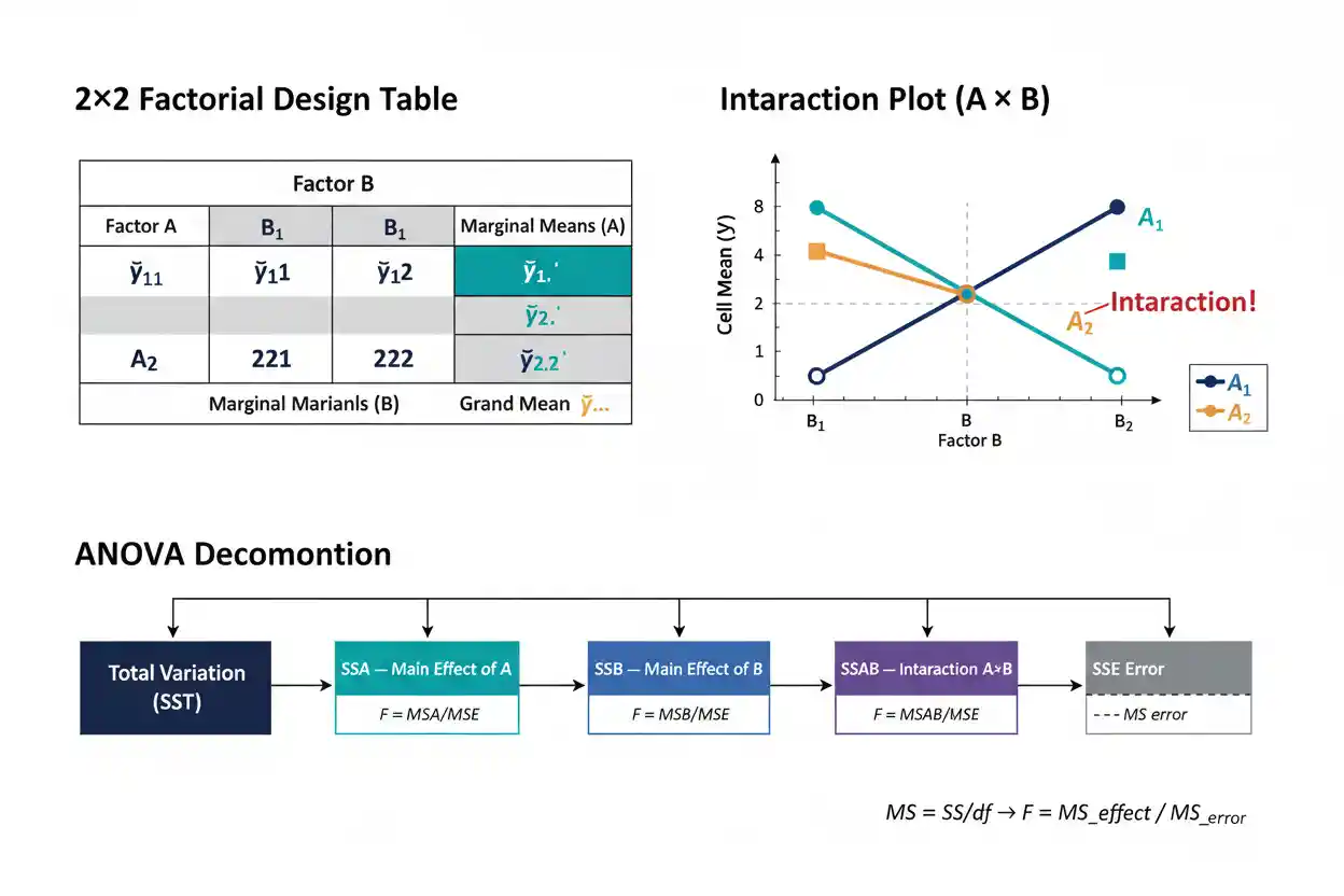
An interaction plot places the levels of one factor on the horizontal axis and uses separate lines for the levels of the other factor.
If the population effects are approximately additive, the lines tend to be approximately parallel.
If the lines are clearly nonparallel, interaction may be present.
Crossing lines can indicate a particularly strong interaction in which the direction of one factor’s effect reverses across levels of the other.
For example:
A1 performs better than A2 under B1
but:
A2 performs better than A1 under B2
would produce a crossover interaction.
An interaction plot is descriptive evidence. Formal inference still requires the appropriate model-based interaction test.
Balanced Two-Way ANOVA
A balanced factorial design has the same number of observations in every factor combination.
Suppose:
Factor A has a levels
Factor B has b levels
each cell contains n observations
Then the total sample size is:
N = abn
Balanced designs make the classical sums-of-squares formulas especially transparent because the factors are represented symmetrically.
The formulas below therefore describe the standard balanced two-way ANOVA with replication.
Unbalanced designs can also be analyzed, but the decomposition requires more care because different definitions of adjusted sums of squares can produce different answers when effects are not orthogonal.
Means Used in Two-Way ANOVA
Let:
ȳᵢⱼ. = mean of cell i,j
ȳᵢ.. = marginal mean for level i of Factor A
ȳ.ⱼ. = marginal mean for level j of Factor B
ȳ… = grand mean across all observations
These means allow total variability to be decomposed into the different factorial components.
The grand mean gives the overall center of the response.
The marginal means describe average levels of each factor.
The cell means contain the information needed to determine whether the two factors combine additively or interact.
Total Sum of Squares
Total variation around the grand mean is:
SST = ΣᵢΣⱼΣₖ(yᵢⱼₖ − ȳ…)²
This measures the total observed response variation before it is assigned to specific model components.
For a balanced two-way ANOVA with interaction:
SST = SSA + SSB + SSAB + SSE
where:
- SSA = sum of squares for Factor A
- SSB = sum of squares for Factor B
- SSAB = interaction sum of squares
- SSE = residual or error sum of squares
The decomposition partitions total variability according to the factorial model.
Sum of Squares for Factor A
For a balanced design:
SSA = bn Σᵢ(ȳᵢ.. − ȳ…)²
The quantity:
ȳᵢ.. − ȳ…
measures how far each Factor A marginal mean lies from the grand mean.
The multiplier:
bn
reflects how many observations contribute to each Factor A marginal mean.
Larger differences among the A marginal means produce a larger SSA.
Sum of Squares for Factor B
Similarly:
SSB = an Σⱼ(ȳ.ⱼ. − ȳ…)²
The term:
ȳ.ⱼ. − ȳ…
measures the deviation of each Factor B marginal mean from the grand mean.
If all B marginal means are similar, SSB will be relatively small.
If they differ substantially, SSB will be larger.
Interaction Sum of Squares
For a balanced design:
SSAB = n ΣᵢΣⱼ(ȳᵢⱼ. − ȳᵢ.. − ȳ.ⱼ. + ȳ…)²
The expression:
ȳᵢⱼ. − ȳᵢ.. − ȳ.ⱼ. + ȳ…
measures how far a cell mean deviates from what would be expected under a purely additive combination of the two factor main effects.
If every cell is well explained by the additive main effects:
SSAB
will be small.
If cell behavior departs substantially from additivity:
SSAB
will increase.
Error Sum of Squares
Within-cell variability is:
SSE = ΣᵢΣⱼΣₖ(yᵢⱼₖ − ȳᵢⱼ.)²
Each observation is compared with the mean of its own factor combination.
This isolates individual variability that remains after accounting for the specific cell mean.
SSE therefore provides the residual variability used as the denominator of the classical F tests.
A smaller SSE means observations cluster more tightly around their corresponding cell means.
A larger SSE means greater unexplained within-cell variability.
Degrees of Freedom
For a balanced two-way ANOVA with:
a Factor A levels
b Factor B levels
n observations per cell
the degrees of freedom are:
dfA = a − 1
dfB = b − 1
dfAB = (a − 1)(b − 1)
dfError = ab(n − 1)
dfTotal = abn − 1
These satisfy:
dfTotal = dfA + dfB + dfAB + dfError
The degrees of freedom determine how each sum of squares is converted into a mean square.
Mean Squares
For Factor A:
MSA = SSA / (a − 1)
For Factor B:
MSB = SSB / (b − 1)
For the interaction:
MSAB = SSAB / [(a − 1)(b − 1)]
For residual error:
MSE = SSE / [ab(n − 1)]
Each effect mean square measures variation associated with that model component per corresponding degree of freedom.
The effect mean squares are then compared with MSE.
F Statistics
The Factor A test statistic is:
FA = MSA / MSE
The Factor B statistic is:
FB = MSB / MSE
The interaction statistic is:
FAB = MSAB / MSE
Each ratio compares effect-related variation with unexplained within-cell variation.
A large F statistic means the corresponding effect mean square is large relative to residual noise.
Under its null hypothesis and the classical model assumptions, each F statistic is evaluated using an F distribution with the appropriate numerator and denominator degrees of freedom.
Worked Two-Way ANOVA Example
Suppose a study evaluates performance under two methods and two environments.
Factor A is Method:
A1
A2
Factor B is Environment:
B1
B2
Three independent observations are collected in every cell.
The scores are:
| Combination | Scores | Cell Mean |
|---|---|---|
| A1B1 | 68, 70, 72 | 70 |
| A1B2 | 78, 80, 82 | 80 |
| A2B1 | 78, 80, 82 | 80 |
| A2B2 | 98, 100, 102 | 100 |
The design is:
2 × 2
with:
n = 3 observations per cell
so:
N = 2 × 2 × 3
N = 12
Step 1: Calculate the Marginal Means
For Factor A:
A1 contains cell means 70 and 80, so:
ȳA1 = (70 + 80)/2
= 75
A2 contains cell means 80 and 100:
ȳA2 = (80 + 100)/2
= 90
Therefore the Factor A marginal means are:
75 and 90
For Factor B:
B1 has:
(70 + 80)/2 = 75
B2 has:
(80 + 100)/2 = 90
So the Factor B marginal means are also:
75 and 90
Step 2: Calculate the Grand Mean
Because the cells contain equal numbers of observations:
ȳ… = (70 + 80 + 80 + 100)/4
= 330/4
= 82.5
The grand mean is:
82.5
Step 3: Calculate SSA
Use:
SSA = bn Σ(ȳᵢ.. − ȳ…)²
Here:
b = 2
n = 3
Therefore:
bn = 6
The deviations are:
75 − 82.5 = −7.5
90 − 82.5 = 7.5
Square them:
(−7.5)² = 56.25
7.5² = 56.25
Then:
SSA = 6(56.25 + 56.25)
SSA = 6(112.5)
SSA = 675
Step 4: Calculate SSB
The Factor B marginal means are also:
75 and 90
and:
an = 2 × 3 = 6
Therefore:
SSB = 6(56.25 + 56.25)
SSB = 675
Step 5: Calculate the Interaction Deviations
Use:
ȳᵢⱼ. − ȳᵢ.. − ȳ.ⱼ. + ȳ…
For A1B1:
70 − 75 − 75 + 82.5
= 2.5
For A1B2:
80 − 75 − 90 + 82.5
= −2.5
For A2B1:
80 − 90 − 75 + 82.5
= −2.5
For A2B2:
100 − 90 − 90 + 82.5
= 2.5
Each squared deviation is:
2.5² = 6.25
There are four cells, so:
Σ interaction deviation² = 4(6.25)
= 25
Multiply by:
n = 3
Therefore:
SSAB = 3(25)
SSAB = 75
Step 6: Calculate SSE
Within every cell, observations differ from the cell mean by:
−2, 0, +2
The squared deviations are:
4, 0, 4
so each cell contributes:
8
There are four cells:
SSE = 4(8)
SSE = 32
Step 7: Calculate Total Sum of Squares
The decomposition gives:
SST = SSA + SSB + SSAB + SSE
SST = 675 + 675 + 75 + 32
SST = 1457
Step 8: Calculate Degrees of Freedom
Because:
a = 2
b = 2
n = 3
we have:
dfA = 2 − 1 = 1
dfB = 2 − 1 = 1
dfAB = (2 − 1)(2 − 1) = 1
dfError = 2 × 2 × (3 − 1)
= 8
and:
dfTotal = 12 − 1
= 11
Check:
1 + 1 + 1 + 8 = 11
Step 9: Calculate Mean Squares
For Factor A:
MSA = 675/1
= 675
For Factor B:
MSB = 675/1
= 675
For the interaction:
MSAB = 75/1
= 75
For residual error:
MSE = 32/8
= 4
Step 10: Calculate the F Statistics
Factor A:
FA = 675/4
= 168.75
Factor B:
FB = 675/4
= 168.75
Interaction:
FAB = 75/4
= 18.75
The ANOVA table is therefore:
| Source | SS | df | MS | F |
|---|---|---|---|---|
| Factor A | 675 | 1 | 675 | 168.75 |
| Factor B | 675 | 1 | 675 | 168.75 |
| A × B Interaction | 75 | 1 | 75 | 18.75 |
| Error | 32 | 8 | 4 | — |
| Total | 1457 | 11 | — | — |
For the interaction:
F(1,8) = 18.75
which corresponds to approximately:
p ≈ 0.0025
The two main-effect F statistics are much larger and also strongly inconsistent with their corresponding equal-marginal-means null hypotheses.
Interpret the Interaction First
The statistically detectable interaction tells us that the environment effect changes by method.
Under A1:
B2 − B1 = 80 − 70
= 10
Under A2:
B2 − B1 = 100 − 80
= 20
Therefore the B effect depends on A.
Likewise, the A effect under B1 is:
80 − 70 = 10
while under B2 it is:
100 − 80 = 20
This is the same interaction viewed from the other direction.
The interaction is symmetric: saying “A’s effect depends on B” and saying “B’s effect depends on A” describe the same departure from additivity.
Interpreting the Main Effects in the Example
The Factor A marginal means are:
A1 = 75
A2 = 90
so the average Factor A difference is:
15
The Factor B marginal means are:
B1 = 75
B2 = 90
so the average Factor B difference is also:
15
These main effects are statistically strong in the example.
However, the interaction shows that neither factor’s effect is exactly 15 at every level of the other factor.
The conditional differences are:
10 in one condition
and:
20 in the other
Therefore, the main effect is an average across heterogeneous conditional effects.
That average can still be useful, but it should not replace the interaction interpretation.
What If There Is No Interaction?
Suppose the cell means instead were:
A1B1 = 70
A1B2 = 80
A2B1 = 80
A2B2 = 90
Then the B effect is:
10
under both A1 and A2.
The A effect is also:
10
under both B1 and B2.
The model is additive.
An interaction contrast is:
(90 − 80) − (80 − 70)
= 10 − 10
= 0
In such a setting, the main effects are easier to summarize because the conditional effects are consistent across the other factor.
Significant Interaction With No Main Effect
It is possible to have a strong interaction while a main effect is close to zero.
Suppose the cell means are:
A1B1 = 60
A1B2 = 90
A2B1 = 90
A2B2 = 60
Both Factor A marginal means are:
75
Both Factor B marginal means are also:
75
so neither main effect exists.
Yet the interaction is dramatic because the direction of the A effect reverses across levels of B.
Under B1:
A2 − A1 = +30
Under B2:
A2 − A1 = −30
Averaging these effects gives zero.
This example shows why “no main effect” does not mean the factor is irrelevant when interaction is present.
Main Effect Without Interaction
A different design might have:
A1B1 = 60
A1B2 = 70
A2B1 = 80
A2B2 = 90
The A difference is:
20
under both B levels.
The B difference is:
10
under both A levels.
The lines on an interaction plot would be parallel.
Both main effects could be substantial while:
interaction = 0
This represents an additive factorial relationship.
Simple Effects
When an interaction is meaningful, analysts often examine simple effects.
A simple effect asks about one factor at a specific level of the other factor.
For the worked example:
Effect of B at A1 = 10
Effect of B at A2 = 20
These are simple effects of B.
Alternatively:
Effect of A at B1 = 10
Effect of A at B2 = 20
These are simple effects of A.
Formal simple-effect tests require appropriate standard errors and multiplicity considerations rather than simply conducting a collection of unplanned tests without adjustment.
Two-Way ANOVA vs Two-Sample T-Test
A Two-Sample T-Test compares two independent population means.
If a study has exactly one categorical factor with two levels, the t-test directly owns that comparison.
Two-way ANOVA instead includes two categorical factors and can test their interaction.
For example:
Treatment A vs Treatment B
alone is a two-group comparison.
But:
Treatment A/B × Location 1/2/3
is a factorial problem because both treatment and location may influence the response and treatment effects may vary by location.
Conducting a separate t-test in every location does not automatically provide the same unified interaction test or overall error structure as a properly specified factorial model.
Two-Way ANOVA vs Two-Sample Z-Test
The Two-Sample Z-Test also addresses a two-group population contrast under a z-based sampling framework.
Two-way ANOVA has a different structure.
Its F tests compare variation attributable to factorial effects with residual variation.
When one factor has exactly two levels, specific ANOVA contrasts can be mathematically related to t tests because:
F with 1 numerator df = t²
under corresponding model conditions.
However, a two-way ANOVA simultaneously represents two factors and their interaction, so reducing the design to isolated z or t tests can discard the factorial structure that motivates the analysis.
Relationship Between F and T
When an ANOVA effect has exactly:
1 numerator degree of freedom
the corresponding F statistic can often be written as:
F = t²
for an equivalent coefficient test within the same linear model and variance assumptions.
For example, if Factor A has exactly two levels:
dfA = 1
Its main-effect F test is equivalent to testing one appropriately coded regression coefficient with a t statistic.
This relationship helps show that ANOVA and regression are not separate mathematical worlds.
They are different presentations of the general linear-model framework.
Two-Way ANOVA as Regression
Categorical factors can be represented using indicator variables and interaction terms.
For a 2×2 design, define:
XA = indicator for Factor A level 2
XB = indicator for Factor B level 2
A regression model can be written:
Y = β₀ + β₁XA + β₂XB + β₃(XA × XB) + ε
Here:
β₀ = mean for the reference cell
β₁ = A difference when B is at its reference level
β₂ = B difference when A is at its reference level
β₃ = interaction or difference-of-differences
For the worked example, the interaction coefficient represents the additional change that makes the A2B2 cell exceed what an additive model would predict.
This regression representation is especially useful for unbalanced data and extensions involving covariates.
Assumption of Independent Observations
Classical two-way ANOVA assumes the errors are independent under the design.
This depends on how the observations were generated.
Suppose 20 measurements are taken from each of ten participants and all 200 rows are treated as independent.
Measurements from the same participant may be correlated.
The ordinary independent-errors ANOVA can then underestimate uncertainty.
Likewise, students nested within classrooms or observations nested within clinics can share common influences.
Repeated-measures, multilevel, or correlated-error methods may be required when the independence structure differs from ordinary factorial sampling.
Normality Assumption
For exact classical small-sample F inference, the model errors are generally assumed to be normally distributed within the factorial model:
εᵢⱼₖ ∼ Normal(0, σ²)
This does not mean the entire pooled response dataset must look like one normal distribution.
Different factor combinations can have different means.
Pooling all observations can therefore create a multimodal-looking overall distribution even when errors within cells are normal.
The relevant diagnostic target is the model’s residual error behavior, not the raw response distribution after ignoring the factors.
Homogeneity of Variance
The classical fixed-effects ANOVA model generally assumes:
Var(εᵢⱼₖ) = σ²
across the cells.
This means each factor combination shares a common residual variance.
If one cell has standard deviation 2 while another has standard deviation 50, the common-variance assumption may be questionable.
Variance inequality can be particularly problematic in unbalanced designs.
Possible responses include using a model with a more appropriate variance structure, transformations when scientifically justified, or robust methods designed for heteroscedastic data.
The correct choice depends on the source and severity of the variance differences.
Outliers
Because ANOVA uses means, sums of squared deviations, and an error variance estimate, unusual observations can materially influence results.
A single extreme response can alter:
- a cell mean
- SSE
- MSE
- factor sums of squares
- F statistics
Potential outliers should therefore be investigated for data quality and model fit.
A valid extreme observation should not be removed merely because the ANOVA becomes more significant without it.
An extreme value can instead signal genuine heavy-tailed variation, a missing subgroup, measurement problems, or an inadequate model.
Residual Diagnostics
After fitting the model, residuals can be examined against fitted values, factor levels, and observation order.
A suitable model should generally avoid strong systematic residual patterns.
For example:
curved or structured residual patterns
can indicate missing model structure,
while:
changing residual spread across groups
can indicate unequal variances.
Time-ordered residual patterns can reveal dependence.
Diagnostics do not prove assumptions perfectly, but they can reveal important departures that a table of F statistics alone cannot show.
Type I Error in Two-Way ANOVA
A Type I Error occurs when an effect null hypothesis is rejected even though that null hypothesis is true.
Two-way ANOVA commonly contains at least three omnibus tests:
Factor A
Factor B
A × B interaction
If each is tested at:
α = 0.05
each individual test has its own nominal false-rejection rate under its corresponding null and valid model.
The probability of at least one false rejection across a broader family of analyses can be larger than 0.05.
Additional post-hoc comparisons can increase the multiplicity issue further.
The error structure should therefore be considered when many follow-up tests are planned.
Type II Error
A Type II Error occurs when the analysis fails to reject a null hypothesis even though the corresponding meaningful effect exists.
For example, an interaction could genuinely exist but remain undetected because:
- the sample is too small
- residual variability is high
- the interaction effect is modest
- the design is highly unbalanced
- measurements are noisy
Failure to reject the interaction null does not prove that the interaction equals exactly zero.
It means the data did not provide sufficient evidence against that null using the specified test.
Confidence intervals or estimated conditional effects can provide additional context about what interaction magnitudes remain plausible.
Statistical Power
Statistical Power is the probability of detecting a specified effect when it is genuinely present.
Power for two-way ANOVA depends on factors including:
- effect magnitude
- residual variance
- sample size per cell
- number of factor levels
- balance of the design
- significance threshold
- the particular main effect or interaction being tested
Interaction effects can require considerable information to estimate precisely because they depend on differences among conditional effects rather than only simple marginal differences.
A study designed with sufficient power for a large main effect is not automatically well powered for a smaller interaction.
Why Interaction Tests Can Need More Data
A main effect can sometimes be estimated by averaging over many observations across the other factor.
An interaction asks whether those factor effects themselves differ.
For a 2×2 design:
interaction = difference of differences
Each component contains sampling uncertainty.
If the true interaction is modest relative to residual variability, the F statistic may remain small even when one or both main effects are easy to detect.
Therefore, factorial studies should be planned around the scientifically important interaction if interaction is central to the research question.
Two-Way ANOVA With Unequal Sample Sizes
Real datasets are often unbalanced.
Suppose cell counts are:
10, 10, 10, and 40
rather than equal.
The simple balanced formulas:
SSA = bnΣ(…)
and:
SSB = anΣ(…)
no longer apply directly in the same way.
In an unbalanced model, factors are not necessarily orthogonal, and different definitions of sums of squares can answer different adjusted questions.
Software may report:
Type I sums of squares
Type II sums of squares
Type III sums of squares
These should not be selected mechanically.
The appropriate hypothesis depends on model hierarchy, interactions, coding, scientific questions, and the design.
Type I Sums of Squares
Type I sums of squares are sequential.
Each model term is evaluated after terms that appeared earlier in the model formula.
Therefore:
order matters
in an unbalanced design.
For example, entering Factor A before Factor B can assign some shared variation to A that might instead be attributed differently if B were entered first.
Sequential sums can be meaningful when factor order has a substantive hierarchical interpretation.
They are not automatically the preferred choice for every observational factorial dataset.
Type II and Type III Sums of Squares
Type II sums of squares generally evaluate main effects after adjusting for other main effects but not interactions in the same way as Type III procedures.
Type III sums of squares evaluate each specified effect after the other terms in the model, subject to the chosen parameterization.
When interactions are present, interpreting adjusted main-effect tests can become subtle because a “main effect” averages or constrains behavior across levels of another factor.
Rather than relying only on a sums-of-squares label, the analysis should identify the actual hypothesis being tested.
Estimated marginal means, contrasts, and simple effects can make those hypotheses clearer.
Model Hierarchy
A common modeling principle is that when an interaction:
A × B
is included, the corresponding lower-order main effects:
A
and:
B
remain in the model.
This hierarchical structure preserves interpretable parameterization and ensures the interaction is defined relative to the constituent factors.
Dropping a main effect while retaining its interaction can create a model whose meaning depends awkwardly on coding and reference values.
Statistical model selection should therefore consider mathematical hierarchy and scientific reasoning rather than deleting terms solely because individual p-values cross a threshold.
Two-Way ANOVA Without Replication
A special spreadsheet-style procedure is sometimes called “two-way ANOVA without replication.”
It contains only one observation for each combination of Factor A and Factor B.
With no replication within cells, the ordinary model cannot separately estimate:
cell-specific interaction variation
from:
residual error
because there is no within-cell replication.
As a result, such a procedure generally relies on an additive model and does not provide the same independent interaction test available in replicated factorial ANOVA.
This limitation is substantial.
If interaction is scientifically important, obtaining replication within factor combinations is generally necessary.
Fixed vs Random Factors
The standard elementary two-way ANOVA usually treats both factors as fixed.
A fixed factor has levels specifically chosen for comparison.
Examples might be:
three named treatments
or:
four specified machine settings
A random factor instead represents levels viewed as sampled from a broader population of possible levels, such as randomly selected schools or operators.
Random and mixed-effects factorial models require different expected mean-square logic or modern mixed-model estimation.
The basic fixed-effects two-way ANOVA formulas should not be applied automatically to random-factor designs.
Post-Hoc Comparisons
If a factor has more than two levels and its omnibus F test is significant, researchers may want to identify which levels differ.
For example, Factor A could have:
A1, A2, A3, A4
The omnibus F test answers whether all four population marginal means can reasonably be treated as equal under the model.
It does not identify which pairs differ.
Post-hoc or planned contrast procedures can address more specific comparisons while accounting for the fact that multiple comparisons increase false-positive opportunities.
When interaction is strong, comparisons within levels of the other factor may be more informative than global marginal pairwise comparisons.
Main Effects Should Not Automatically Be Ignored When Interaction Exists
A common oversimplification says:
“If interaction is significant, never interpret main effects.”
That is too absolute.
A main effect still describes an average contrast across the levels represented in the design.
The real issue is whether that average meaningfully summarizes the conditional effects.
If every conditional effect points in the same direction but varies in size, an average effect can still be useful when clearly described.
If effects reverse direction, the average may be highly misleading.
Interpretation should therefore follow the actual interaction pattern rather than a rigid rule.
Statistical Significance vs Practical Importance
Suppose a very large factorial experiment estimates an interaction corresponding to only:
0.05 response units
but produces:
p < 0.001
The interaction may be statistically detectable yet practically irrelevant.
Alternatively, a smaller experiment might estimate a large conditional difference but have a wide confidence interval and nonsignificant interaction test.
F statistics and p-values describe evidence relative to sampling uncertainty.
They do not define the real-world importance of an effect.
Cell means, contrasts, effect sizes, and confidence intervals should accompany significance tests whenever magnitude matters.
Effect Sizes in Two-Way ANOVA
ANOVA effect magnitude can be summarized in several ways.
One common sample-based measure is eta squared:
η²effect = SSeffect / SST
Partial eta squared is:
partial η²effect = SSeffect / (SSeffect + SSE)
These quantities describe proportions of observed sum-of-squares variation under particular definitions.
For the worked interaction:
SSAB = 75
SSE = 32
so:
partial η²AB = 75 / (75 + 32)
= 75/107
≈ 0.701
This is very large in the constructed example.
However, effect-size interpretation depends on field, design, and estimator properties. A proportion-of-variance statistic should not replace examination of the actual cell means and conditional differences.
Common Two-Way ANOVA Mistakes
A common mistake is examining only the main-effect p-values while ignoring the interaction. If interaction is present, averaged factor effects can obscure meaningful conditional differences.
Another mistake is conducting numerous separate Two-Sample T-Test comparisons instead of fitting the factorial model. Separate comparisons do not automatically provide a test of interaction and can inflate multiplicity.
Researchers also sometimes treat repeated observations from the same person as independent, use balanced-design formulas on substantially unbalanced data, or assume equal sample sizes guarantee equal variances.
Another error is interpreting:
p > 0.05
as proof that a factor has no effect.
Finally, statistical significance should not be interpreted as causation unless the study design and assumptions support a causal conclusion.
How to Calculate Two-Way ANOVA
For a balanced replicated design, first organize observations by the combinations of Factor A and Factor B.
Calculate:
cell means ȳᵢⱼ.
then:
Factor A marginal means ȳᵢ..
Factor B marginal means ȳ.ⱼ.
and:
grand mean ȳ…
Calculate:
SSA = bnΣᵢ(ȳᵢ.. − ȳ…)²
SSB = anΣⱼ(ȳ.ⱼ. − ȳ…)²
SSAB = nΣᵢΣⱼ(ȳᵢⱼ. − ȳᵢ.. − ȳ.ⱼ. + ȳ…)²
SSE = ΣᵢΣⱼΣₖ(yᵢⱼₖ − ȳᵢⱼ.)²
Then determine the corresponding degrees of freedom and mean squares.
Finally calculate:
FA = MSA/MSE
FB = MSB/MSE
FAB = MSAB/MSE
and use the corresponding F distributions to evaluate the three null hypotheses.
How to Interpret a Two-Way ANOVA
A useful interpretation usually starts with the interaction.
If the interaction is substantial, describe how the effect of one factor differs across levels of the other factor.
For example:
The difference between B1 and B2 was approximately 10 units under A1 but approximately 20 units under A2.
Then describe the main effects as marginal averages if they remain useful:
Averaged across B levels, A2 exceeded A1 by approximately 15 units.
Averaged across A levels, B2 exceeded B1 by approximately 15 units.
This wording keeps the distinction between conditional and marginal effects explicit.
How to Report Two-Way ANOVA
A strong report should identify:
- factor structure
- cell means or estimated marginal means
- interaction F statistic
- main-effect F statistics
- numerator and denominator degrees of freedom
- p-values
- relevant effect sizes or confidence intervals
For the worked example:
Factor A: F(1,8) = 168.75
Factor B: F(1,8) = 168.75
A × B interaction: F(1,8) = 18.75, p ≈ 0.0025
The interaction should then be interpreted using the cell means rather than simply stating that it was significant.
The substantive information is that the B difference changes from 10 units at A1 to 20 units at A2.
Frequently Asked Questions
What is two-way ANOVA?
Two-way ANOVA analyzes a quantitative response using two categorical factors and can test both factor main effects and their interaction.
What does two-way mean?
It means the model contains two explanatory factors.
What does ANOVA test in a two-way design?
It commonly tests:
Factor A main effect
Factor B main effect
Factor A × Factor B interaction
What is the two-way ANOVA model?
A common fixed-effects model is:
Yᵢⱼₖ = μ + αᵢ + βⱼ + (αβ)ᵢⱼ + εᵢⱼₖ
What is an interaction?
An interaction means the effect of one factor depends on the level of the other factor.
What is a main effect?
A main effect is an average difference among the marginal means of one factor across the levels of the other factor.
What is the interaction formula in a 2×2 design?
A useful difference-of-differences representation is:
(μ₂₂ − μ₂₁) − (μ₁₂ − μ₁₁)
What does a zero interaction mean?
It means the factor effects are additive according to that interaction contrast.
Can an interaction exist without main effects?
Yes. Strong crossover interactions can produce identical marginal means even when conditional effects are large.
Can main effects exist without interaction?
Yes. Factor effects can be consistent across the levels of the other factor.
What is the sum-of-squares decomposition?
For a balanced replicated design:
SST = SSA + SSB + SSAB + SSE
What are the degrees of freedom?
For a levels of A, b levels of B, and n observations per cell:
dfA = a−1
dfB = b−1
dfAB = (a−1)(b−1)
dfError = ab(n−1)
What is the F statistic for Factor A?
FA = MSA/MSE
What is the F statistic for the interaction?
FAB = MSAB/MSE
Should interaction be interpreted before main effects?
Usually it should be examined first because interaction determines whether averaged main effects adequately summarize the conditional relationships.
Does significant interaction make main effects meaningless?
Not necessarily. Main effects remain marginal averages, but their usefulness depends on whether those averages meaningfully summarize the conditional effects.
What assumptions does classical two-way ANOVA make?
Important conditions include appropriate independence, a quantitative response, suitable model form, approximately normal errors for exact small-sample inference, and a common residual variance in the classical homoscedastic model.
Does the entire outcome distribution have to be normal?
No. The normality assumption concerns model errors or within-model residual behavior, not necessarily the pooled raw responses across groups with different means.
Does equal sample size guarantee equal variance?
No.
Can two-way ANOVA handle unequal sample sizes?
Yes, through the general linear-model framework, but sums-of-squares definitions and effect hypotheses require more care than in a balanced design.
What is two-way ANOVA without replication?
It is a design with one observation per factor combination. Without within-cell replication, ordinary interaction and residual error cannot generally be separately estimated.
What is the difference between two-way ANOVA and a two-sample t-test?
A two-sample t-test compares two independent population means. Two-way ANOVA contains two factors and can test their interaction.
Is two-way ANOVA related to regression?
Yes. Categorical factors can be represented with indicator variables and interaction terms in a linear regression model.
Does a significant ANOVA prove causation?
No. Causal interpretation depends on the design, such as valid random assignment and other required assumptions.
What does a nonsignificant interaction mean?
It means the analysis did not provide sufficient evidence against the no-interaction null. It does not prove the interaction is exactly zero.
What affects power for an interaction?
Sample size, interaction magnitude, residual variability, balance, factor levels, and significance threshold all affect interaction-test power.
Key Takeaway
Two-way ANOVA analyzes a quantitative response across two categorical factors while separating three distinct inferential questions:
Factor A main effect
Factor B main effect
Factor A × Factor B interaction
For a balanced replicated model:
Yᵢⱼₖ = μ + αᵢ + βⱼ + (αβ)ᵢⱼ + εᵢⱼₖ
and total variation is partitioned as:
SST = SSA + SSB + SSAB + SSE
The corresponding F tests are:
FA = MSA/MSE
FB = MSB/MSE
FAB = MSAB/MSE
The interaction is the defining feature of the factorial analysis because it determines whether one factor has the same effect across the levels of the other factor. In a 2×2 design, it can be understood as a difference of differences.
In the worked example, both factors had average 15-unit main effects, but the conditional factor difference changed from 10 to 20 units. The interaction test therefore revealed information that the marginal means alone could not show.
Reliable two-way ANOVA interpretation requires more than comparing three p-values. The factor design, cell means, interaction pattern, residual variability, independence structure, variance assumptions, effect magnitude, statistical power, and study design all determine what conclusions the analysis can support. When these elements are handled appropriately, two-way ANOVA provides a compact and powerful framework for understanding not only whether two factors matter, but whether they matter differently when they occur together.