Regression Intercept: Definition, Formula & Example

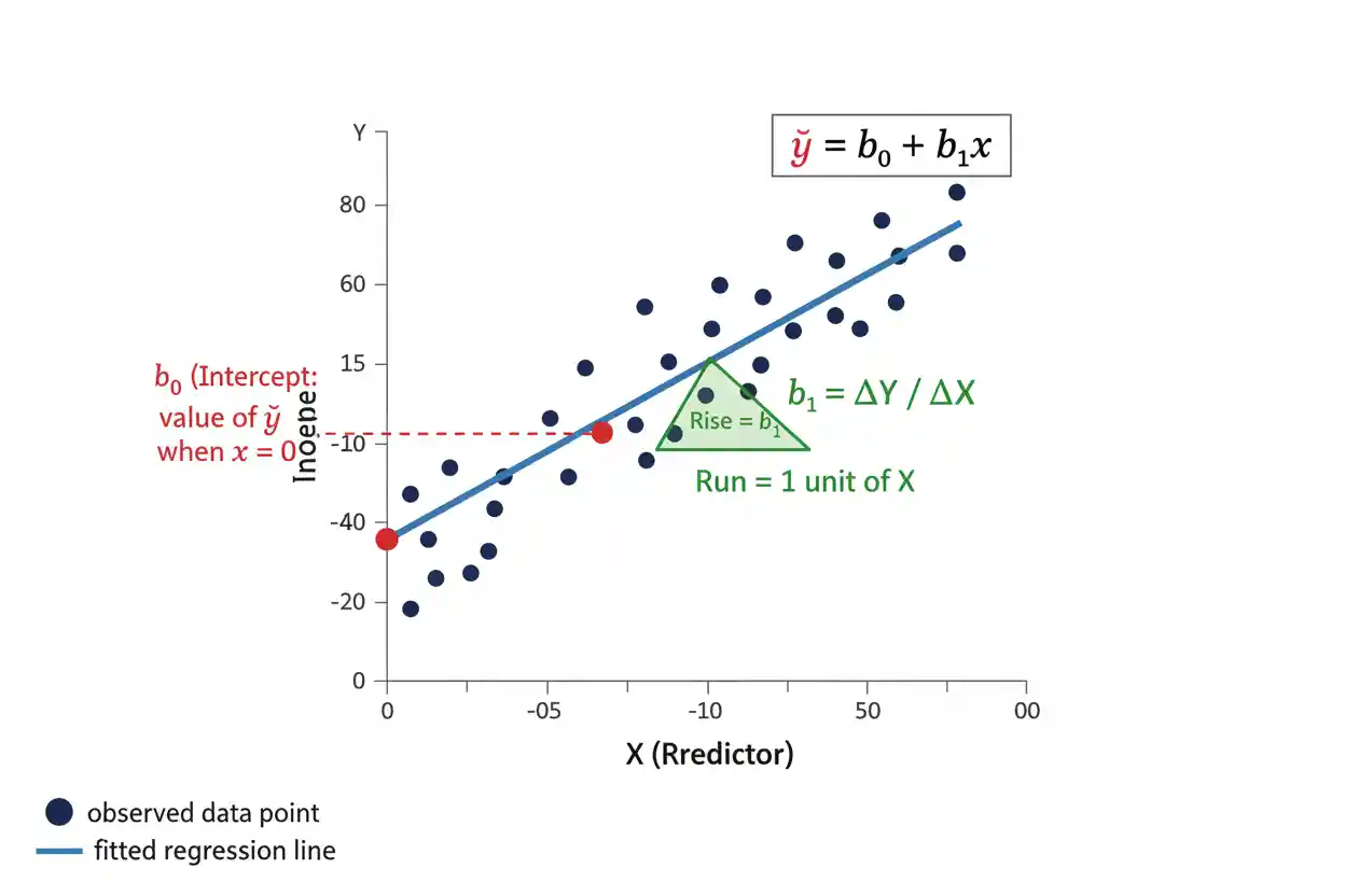
The regression intercept is the constant term in a regression equation and represents the model’s predicted response when all numerical predictors equal zero and categorical predictors are at their reference levels. In a simple linear regression written as ŷ = b₀ + b₁x, the intercept b₀ is the fitted value of Y at x = 0, while b₁ determines how the fitted response changes as x changes. The intercept is mathematically necessary in most ordinary regression models because it establishes the vertical position of the fitted line or regression surface, but its substantive interpretation depends heavily on how the predictors are measured and coded. If x = 0 is realistic and appears within or near the observed data, the intercept may have a clear practical meaning. If zero is impossible, arbitrary, or far outside the observed predictor range, the intercept may still be essential to the fitted equation without representing a meaningful real-world condition. Centering predictors can often make the intercept more interpretable without changing fitted values or the slope structure of an equivalent linear model.

In multiple regression, the intercept refers to the simultaneous zero/reference configuration of all predictors, so careless interpretation can produce statements about a predictor combination that never occurs in the data. The intercept can also be estimated, tested, and assigned a confidence interval like other regression coefficients, although testing whether it equals zero is often much less substantively important than estimating the relationships represented by other coefficients.

The regression intercept is a foundational concept within Statistics & Probability and Inference & Regression. Understanding it correctly requires separating the model’s vertical baseline from the change represented by the Regression Slope.

What Is a Regression Intercept?

In simple linear regression, the fitted equation is:

ŷ = b₀ + b₁x

where:

• ŷ = predicted value of the response
• b₀ = estimated regression intercept
• b₁ = estimated regression slope
• x = predictor value

Setting:

x = 0

gives:

ŷ = b₀ + b₁(0)

so:

ŷ = b₀

Therefore, b₀ is the predicted response when x equals zero.

The population model is commonly written:

Y = β₀ + β₁X + ε

Here:

β₀ = population intercept

while:

b₀ = sample estimate of β₀

The distinction matters because β₀ is an unknown population parameter, whereas b₀ is calculated from observed sample data.

Regression Intercept Formula

For ordinary simple linear regression with an intercept, the estimated slope is:

b₁ = Σ[(xᵢ − x̄)(yᵢ − ȳ)] / Σ(xᵢ − x̄)²

Once b₁ has been estimated, the intercept is:

b₀ = ȳ − b₁x̄

This formula ensures that the fitted ordinary least squares line passes through the point:

(x̄, ȳ)

Substituting x̄ into the fitted equation:

ŷ = b₀ + b₁x̄

and replacing b₀ with:

ȳ − b₁x̄

gives:

ŷ = ȳ − b₁x̄ + b₁x̄

so:

ŷ = ȳ

Thus the ordinary least squares regression line with an intercept always passes through the sample means of X and Y.

Worked Regression Intercept Example

Suppose a fitted regression predicts weekly sales from advertising expenditure:

ŷ = 20 + 4x

where x measures advertising expenditure in thousands of currency units.

The regression intercept is:

b₀ = 20

The slope is:

b₁ = 4

At:

x = 0

the prediction is:

ŷ = 20 + 4(0)

ŷ = 20

Therefore, the fitted model predicts weekly sales of 20 units when advertising expenditure equals zero.

At:

x = 5

the prediction becomes:

ŷ = 20 + 4(5)

ŷ = 40

The intercept establishes the baseline position of the fitted line, while the slope determines how that predicted value changes as advertising expenditure increases.

Intercept vs Slope

The intercept and slope play distinct roles.

For:

ŷ = 20 + 4x

the intercept:

b₀ = 20

describes the fitted value when:

x = 0

The slope:

b₁ = 4

describes the estimated change in ŷ for a one-unit increase in x.

Graphically, the intercept determines where the regression line crosses the y-axis, while the slope determines its steepness and direction.

Changing only the intercept shifts the regression line vertically without changing its slope.

Changing only the slope rotates the line around the location implied by the other model parameters.

These concepts are related but should not be interpreted interchangeably.

Graphical Meaning of the Intercept

On a conventional regression graph, the horizontal axis represents X and the vertical axis represents Y.

The fitted line is:

ŷ = b₀ + b₁x

At the y-axis:

x = 0

Therefore, the line crosses the y-axis at:

y = b₀

If:

b₀ = 10

the fitted line crosses at:

(0, 10)

If:

b₀ = −5

it crosses at:

(0, −5)

A negative intercept is not automatically an error. It simply means the mathematical regression line predicts a negative value at x = 0.

Whether that prediction is realistic depends on the context and whether x = 0 is a meaningful predictor value.

Why the Intercept Can Be Meaningful

Consider a model predicting electricity usage from the number of operating hours:

ŷ = 15 + 2.8x

If:

x = operating hours

then:

b₀ = 15

may represent baseline electricity consumption when the measured equipment is not operating.

If background systems continue consuming electricity at zero operating hours, the intercept has a natural practical interpretation.

Likewise, a model predicting total cost from production quantity might have:

Cost = fixed cost + variable cost per unit × quantity

Here, the intercept can represent estimated fixed cost at zero production.

In such situations, zero is both meaningful and relevant, making the intercept substantively useful.

When the Intercept Has Little Practical Meaning

Suppose a regression predicts adult blood pressure from age using observations only from people aged 40 to 80:

ŷ = 75 + 0.6x

Mathematically:

b₀ = 75

is the predicted response at:

age = 0

But newborn age lies completely outside the population and data range represented by the study.

The intercept remains necessary for positioning the fitted line over ages 40 to 80, but interpreting 75 as a meaningful predicted blood pressure for a newborn would be inappropriate.

The distinction is important:

mathematical interpretation ≠ necessarily useful substantive interpretation

Every ordinary intercept has a mathematical definition, but not every intercept describes a realistic condition.

Extrapolation and the Intercept

An intercept can effectively represent an extrapolated prediction when zero lies far outside the observed predictor values.

Suppose the available X values range from:

500 to 1,000

but the fitted equation is:

ŷ = 200 + 0.7x

The intercept:

200

corresponds to x = 0, hundreds of units outside the observed range.

The fitted line may describe the relationship well between 500 and 1,000 while being unreliable at zero.

Therefore, the intercept should not automatically be interpreted as a scientifically valid prediction at x = 0.

Regression coefficients are mathematical components of the fitted model, but substantive conclusions should remain anchored to predictor values supported by the data and model assumptions.

How the Intercept Is Calculated From Means

Consider data with:

x̄ = 10

ȳ = 50

and estimated slope:

b₁ = 3

The intercept is:

b₀ = ȳ − b₁x̄

Substitute the values:

b₀ = 50 − 3(10)

b₀ = 50 − 30

b₀ = 20

The fitted equation is:

ŷ = 20 + 3x

At the sample mean:

x = 10

the prediction is:

ŷ = 20 + 3(10)

ŷ = 50

which equals:

ȳ = 50

This demonstrates the geometric property that the fitted OLS line with an intercept passes through:

(x̄, ȳ)

Another Worked Example

Suppose a regression predicting exam score from study hours has:

x̄ = 6

ȳ = 72

and:

b₁ = 4

Calculate the intercept:

b₀ = 72 − 4(6)

b₀ = 72 − 24

b₀ = 48

The fitted model is:

ŷ = 48 + 4x

At:

x = 0

the predicted score is:

ŷ = 48

At:

x = 5

the predicted score is:

ŷ = 48 + 4(5)

ŷ = 68

At:

x = 10

the predicted score is:

ŷ = 48 + 4(10)

ŷ = 88

Here, the intercept represents the model’s estimated exam score at zero study hours. Whether that is substantively meaningful depends on whether students with zero study hours are reasonably represented by the population and data used to fit the model.

Population Intercept vs Estimated Intercept

The population regression model may be written:

E(Y | X = x) = β₀ + β₁x

The population intercept is:

β₀

It represents the true conditional mean of Y at X = 0 under the specified population model.

Because population parameters are generally unknown, sample data are used to estimate:

β₀ with b₀

Different random samples will usually produce different values of b₀.

Therefore:

b₀ ≠ β₀

in general.

Instead, b₀ is an estimator-derived estimate subject to sampling uncertainty.

This uncertainty can be summarized using its standard error, confidence interval, or an appropriate statistical test.

Intercept in Multiple Regression

For multiple linear regression:

ŷ = b₀ + b₁x₁ + b₂x₂ + … + bₖxₖ

the intercept represents the predicted response when:

x₁ = 0

x₂ = 0

…

xₖ = 0

for all numerical predictors, while categorical predictors are represented according to their reference coding.

Suppose:

ŷ = 30 + 2x₁ − 4x₂

Then:

b₀ = 30

means the model predicts:

ŷ = 30

when:

x₁ = 0

and:

x₂ = 0

The important question is whether that simultaneous zero configuration is meaningful or represented by the data.

In a model with many predictors, the intercept can correspond to an artificial combination that never actually occurs.

Intercept With Categorical Predictors

Categorical predictors are typically represented using indicator variables.

Suppose a regression models salary using experience and department:

ŷ = b₀ + b₁Experience + b₂DepartmentB

where:

DepartmentB = 1 for Department B

and:

DepartmentB = 0 for reference Department A

Then the intercept b₀ represents the predicted salary for:

Experience = 0

and:

Department = A

The intercept therefore combines the zero value of continuous predictors with the reference levels of categorical predictors.

If several categorical variables are included, the intercept corresponds to the combination of all reference categories.

Understanding reference coding is essential before giving the intercept a practical interpretation.

Categorical Example

Suppose:

ŷ = 35 + 2.5Experience + 8Manager

where:

Manager = 1 for managers

Manager = 0 for non-managers

The intercept is:

b₀ = 35

This predicts:

ŷ = 35

for a non-manager with zero years of experience.

For a manager with zero years:

ŷ = 35 + 8

ŷ = 43

The coefficient 8 changes the predicted baseline between the two categories, while the regression intercept remains tied to the chosen reference category.

If the category coding were reversed, the intercept would change even though the model could produce identical fitted values.

Coding Changes the Intercept

Regression coefficients depend on how predictors are coded.

Suppose a categorical variable has:

0 = Control

1 = Treatment

Then the intercept corresponds to the Control group.

If the coding is reversed:

0 = Treatment

1 = Control

the intercept becomes the predicted response for the Treatment group instead.

The fitted predictions can remain exactly the same, but the numerical intercept and interpretation change.

This illustrates a broader principle:

the intercept is parameterization-dependent

It is not an intrinsic descriptive constant independent of the way the model is expressed.

Centering a Predictor

A common way to improve intercept interpretation is to center a predictor.

Define:

Xc = X − x̄

The centered predictor has sample mean:

X̄c = 0

Now fit:

ŷ = b₀,c + b₁Xc

When:

Xc = 0

we have:

X = x̄

Therefore, the centered intercept represents the predicted response at the average observed predictor value rather than at the original X = 0.

This can make the intercept much more interpretable.

Centering Example

Suppose the original model is:

ŷ = 20 + 3x

and:

x̄ = 10

Define:

xc = x − 10

Since:

x = xc + 10

substitute into the model:

ŷ = 20 + 3(xc + 10)

ŷ = 20 + 3xc + 30

ŷ = 50 + 3xc

The centered model is:

ŷ = 50 + 3xc

The intercept changes from:

20

to:

50

while the slope remains:

3

and every fitted value remains unchanged.

The new intercept 50 represents the fitted response at:

x = 10

which is the sample mean of X.

Centering Does Not Change the Underlying Fit

In an ordinary linear model with an intercept, merely subtracting a constant from a predictor and refitting the equivalent model does not change:

• fitted values
• residuals
• residual sum of squares
• overall model fit
• slope associated with that predictor in the simple additive case

It changes the coordinate system used to express the regression equation.

The intercept changes because the meaning of predictor zero changes.

This makes centering especially useful when the original zero value is arbitrary or outside the meaningful data range.

Centering Multiple Predictors

Suppose:

ŷ = b₀ + b₁x₁ + b₂x₂

and both predictors are centered:

x₁c = x₁ − x̄₁

x₂c = x₂ − x̄₂

The centered intercept corresponds to the fitted response when:

x₁ = x̄₁

and:

x₂ = x̄₂

rather than when both predictors equal their original zero values.

This can turn an obscure intercept into an estimated response for an observation with average predictor values.

However, if interactions or nonlinear terms are present, coefficient interpretation requires additional care because re-centering can change the meanings of lower-order terms even though the model’s fitted predictions remain equivalent when transformed correctly.

Intercept With Interaction Terms

Consider:

ŷ = b₀ + b₁x₁ + b₂x₂ + b₃x₁x₂

The intercept b₀ still represents the predicted response when:

x₁ = 0

and:

x₂ = 0

But the lower-order coefficients now have conditional interpretations tied to zero values of the interacting variables.

For example, b₁ represents the slope of x₁ when:

x₂ = 0

If x₂ = 0 is not meaningful, both the intercept and lower-order slope interpretation can become awkward.

Centering an interacting continuous predictor around a meaningful value can therefore improve interpretation.

The intercept remains the model’s baseline under the chosen coding.

Intercept With Polynomial Terms

Suppose a quadratic regression is:

ŷ = b₀ + b₁x + b₂x²

At:

x = 0

both:

x = 0

and:

x² = 0

so:

ŷ = b₀

The intercept therefore retains its basic interpretation as the fitted response at zero.

However, the overall relationship is curved, so the intercept should not be interpreted independently of the full model when discussing predictions away from zero.

The constant term locates the curve vertically; it does not by itself describe the shape.

Intercept and Residuals

A residual is:

eᵢ = yᵢ − ŷᵢ

The intercept contributes to every fitted value:

ŷᵢ = b₀ + b₁xᵢ

so changing b₀ while holding the slope fixed shifts all fitted values and changes the residuals.

In ordinary least squares regression with an intercept, an important property is:

Σeᵢ = 0

apart from numerical rounding.

This means:

mean residual = 0

The intercept helps ensure that the fitted model is vertically positioned so positive and negative residual deviations balance in this algebraic sense.

The broader interpretation and diagnostic use of these errors are covered in Residuals.

Why Residual Mean Is Zero With an Intercept

OLS minimizes:

SSE = Σ(yᵢ − b₀ − b₁xᵢ)²

One first-order condition for minimizing this expression with respect to b₀ produces:

Σ(yᵢ − ŷᵢ) = 0

Therefore:

Σeᵢ = 0

This property generally depends on including an intercept.

If the regression is forced through the origin, residuals do not necessarily sum to zero.

This is one reason models without an intercept behave differently from ordinary regression models with a freely estimated constant.

Regression Through the Origin

A no-intercept regression has the form:

ŷ = b₁x

This forces:

ŷ = 0 when x = 0

Rather than estimating the intercept from the data, the model imposes:

β₀ = 0

as a structural constraint.

This should not be done merely because the estimated intercept is statistically nonsignificant.

Removing the intercept changes the regression geometry, slope estimate, residual properties, sums-of-squares decomposition, and potentially the interpretation of R².

A no-intercept model should generally be used only when substantive theory and measurement scales justify the requirement that the response truly equals zero when all predictors equal zero.

Why a Nonsignificant Intercept Does Not Mean Remove It

Suppose a test of:

H₀: β₀ = 0

produces:

p = 0.40

This means the data do not provide strong evidence against a zero intercept under the specified model and test.

It does not imply that β₀ should automatically be constrained to zero.

The intercept often serves an important structural function even when zero is a plausible population value.

Removing it imposes an exact restriction rather than simply acknowledging uncertainty.

Model specification should be driven by theory, design, and predictive consequences rather than deleting the constant solely because its P-Value exceeds a conventional significance threshold.

Testing the Regression Intercept

The population intercept can be tested using:

H₀: β₀ = β₀,0

For the common zero-null test:

H₀: β₀ = 0

A conventional t statistic is:

t = b₀ / SE(b₀)

More generally:

t = (b₀ − β₀,0) / SE(b₀)

Suppose:

b₀ = 10

and:

SE(b₀) = 4

Then:

t = 10 / 4

t = 2.5

The statistic is evaluated using the appropriate t reference distribution under the regression assumptions.

Whether testing β₀ = 0 is substantively useful depends on whether zero has meaningful relevance in the predictor coding.

Confidence Interval for the Regression Intercept

A classical confidence interval for β₀ has the general form:

b₀ ± t* × SE(b₀)

Suppose:

b₀ = 20

SE(b₀) = 5

and:

t* = 2.0

Then:

Margin = 2.0 × 5

Margin = 10

The interval is:

20 ± 10

or:

10 to 30

This interval describes uncertainty in the population intercept under the model and interval procedure.

It does not describe the range of future Y observations at x = 0.

That predictive question requires a Prediction Interval, which includes individual outcome variability in addition to uncertainty in the fitted mean.

Intercept Confidence Interval vs Prediction Interval

Suppose:

b₀ = 20

A 95% confidence interval for β₀ might be:

15 to 25

while a 95% prediction interval for a future observation at x = 0 might be:

2 to 38

These intervals have different targets.

The confidence interval concerns:

E(Y | X = 0)

through the population intercept.

The prediction interval concerns:

a new individual Y observation when X = 0

Individual responses vary around their mean, so the prediction interval is ordinarily much wider.

A narrow confidence interval for the intercept therefore does not imply that individual outcomes at zero can be predicted precisely.

Standard Error of the Intercept

In simple OLS regression with homoscedastic errors, the estimated standard error of b₀ has the structure:

SE(b₀) = sₑ × √[1/n + x̄² / Σ(xᵢ − x̄)²]

where sₑ is the residual standard error.

This formula shows why the intercept can be estimated imprecisely when zero lies far from the center of the observed X data.

If x̄ is large relative to the spread of X around its mean, the term:

x̄² / Σ(xᵢ − x̄)²

can be large.

Centering X makes the new predictor mean zero and can substantially reduce the standard error of the redefined intercept because the new intercept represents the mean response at the center of the data rather than an extrapolated value at the original zero.

Why Intercept Uncertainty Can Be Large

Suppose all observed x-values lie near 1,000.

The regression line may be estimated quite well over the region:

950 to 1,050

but the intercept asks what the line predicts at:

x = 0

Estimating that point requires extending the fitted line far from the observed data.

Even a small amount of uncertainty in the slope can create substantial uncertainty in the predicted value at zero when zero is distant from x̄.

This is why a regression can have highly precise fitted values near the data center while having a poorly estimated original-scale intercept.

Standardizing Predictors

Suppose a predictor is standardized:

zX = (X − x̄) / sX

Then:

zX = 0

corresponds to:

X = x̄

A regression using zX therefore has an intercept corresponding to the predicted response at the average original X value.

If Y remains in its original units, the intercept remains in Y units.

If both X and Y are standardized and a standard OLS regression with intercept is fitted, the sample means are zero, so the estimated intercept is ordinarily:

b₀ = 0

subject to numerical precision.

This result arises from centering, not because all regression intercepts are inherently zero.

Units of the Intercept

The regression intercept has the same units as the response variable Y.

If Y is measured in dollars:

b₀ is measured in dollars

If Y is measured in kilograms:

b₀ is measured in kilograms

If Y is a test score:

b₀ is measured in score points

This differs from a slope, whose units are:

Y units per X unit

For example, in:

ŷ = 100 + 5x

if Y is dollars and X is hours, then:

intercept = 100 dollars

while:

slope = 5 dollars per hour

The distinction helps prevent misinterpretation of coefficient magnitudes.

Negative Regression Intercept

A negative intercept is mathematically valid.

Suppose:

ŷ = −10 + 4x

Then:

b₀ = −10

At:

x = 0

the model predicts:

ŷ = −10

If Y can meaningfully take negative values, this may be perfectly reasonable.

If Y cannot be negative, such as physical quantity constrained above zero, the intercept may still be acceptable when x = 0 lies outside the relevant predictor range.

The model’s usefulness should be assessed over the region where predictions are needed rather than rejecting it solely because the extrapolated intercept violates a practical constraint.

Intercept Equal to Zero

An estimated intercept can equal or be close to zero.

For:

ŷ = 0 + 2x

the fitted line passes through the origin.

This may happen naturally without forcing the model through zero.

There is an important distinction between:

estimated b₀ ≈ 0

and:

imposing b₀ = 0

The first is a result obtained from an unconstrained model.

The second is a modeling restriction that changes the estimation problem.

A small estimated intercept is not by itself a reason to replace the first model with the second.

Intercept-Only Model

A regression model can contain only an intercept:

Yᵢ = β₀ + εᵢ

The OLS estimate is:

b₀ = ȳ

Thus an intercept-only model predicts the same value for every observation:

ŷᵢ = ȳ

This model forms an important baseline for regression because more complex models are often compared against the mean-only prediction.

It also illustrates that the intercept is not merely a graphical y-axis crossing. It can represent the entire expected-value structure when no predictors are included.

Connection to the Paired T-Test

After a paired dataset is transformed into within-pair differences Dᵢ, the Paired T-Test can be represented as an intercept-only model:

Dᵢ = β₀ + εᵢ

In that representation:

β₀ = μD

the population mean paired difference.

Testing:

H₀: μD = 0

is equivalent under corresponding assumptions to testing:

H₀: β₀ = 0

in the intercept-only model.

This connection demonstrates how the same regression parameter concept appears across seemingly different statistical procedures.

The paired t-test still retains its own substantive interpretation as inference about within-pair differences.

Intercept and the Mean of Y

In an intercept-only OLS model:

b₀ = ȳ

In a simple regression with a centered predictor:

xc = x − x̄

the fitted intercept also equals:

b₀,c = ȳ

because:

x̄c = 0

and:

b₀,c = ȳ − b₁(0)

b₀,c = ȳ

This makes centered regression particularly intuitive: the intercept gives the fitted response at the average predictor value and equals the sample mean of Y in ordinary simple OLS.

Intercept in Models With Several Centered Predictors

Consider:

ŷ = b₀ + b₁x₁c + b₂x₂c

where both predictors have been centered around their sample means.

At:

x₁c = 0

and:

x₂c = 0

the prediction is:

ŷ = b₀

Under ordinary additive OLS with an intercept, this corresponds to the fitted response at the simultaneous predictor means.

This baseline often has substantially more practical meaning than a prediction for all original predictors equal to zero.

However, an observation exactly at every predictor mean need not actually exist in the dataset. The interpretation remains model-based.

Intercept and Dummy-Variable Reference Groups

Suppose a model includes:

ŷ = b₀ + b₁Age + b₂GroupB + b₃GroupC

with Group A omitted as the reference category.

The intercept represents the fitted response for:

Group A

at:

Age = 0

If Age is centered around 40:

Agec = Age − 40

then the intercept becomes the fitted response for:

Group A at age 40

This is often much easier to interpret.

Changing the reference category would change the intercept again while leaving the model’s complete set of fitted predictions unchanged.

The meaning of b₀ is therefore inseparable from predictor coding.

Intercept in Logistic Regression

In a logistic model:

log[p / (1 − p)] = β₀ + β₁x

the intercept β₀ represents the log-odds of the event when x = 0.

The corresponding baseline odds are:

Odds₀ = e^(β₀)

and baseline probability is:

p₀ = 1 / (1 + e^(−β₀))

Thus the general baseline concept remains, although the scale differs from ordinary linear regression.

In linear regression, the intercept is on the response scale.

In logistic regression, it is on the log-odds scale before transformation.

This distinction shows why regression coefficients must always be interpreted in relation to the model’s link and outcome structure.

Intercept in Other Regression Models

Regression models can use different response distributions and link functions, so the constant term does not always directly represent the expected outcome on the original response scale.

In a generalized linear model, the intercept usually represents the model’s linear predictor when all predictors equal zero or are at reference levels.

A transformation through the model’s inverse link may be required to express the baseline prediction on a more familiar scale.

Therefore, although the concept of a baseline constant generalizes broadly, the familiar statement:

intercept = predicted Y at X = 0

applies directly to ordinary linear regression and must be adapted carefully for other model families.

Does the Intercept Affect Predictions?

Yes.

Every prediction from:

ŷ = b₀ + b₁x

contains b₀.

Suppose two models have the same slope:

Model A: ŷ = 10 + 3x

Model B: ŷ = 20 + 3x

At every common x-value:

Prediction from Model B − Prediction from Model A = 10

The two lines are parallel, but Model B lies ten response units higher everywhere.

The intercept therefore affects the level of all fitted predictions, not only the prediction at zero.

Does a Large Intercept Mean a Strong Relationship?

No.

The magnitude of the intercept does not measure the strength of association between X and Y.

Consider:

ŷ = 1,000,000 + 0.01x

The intercept is enormous, while the slope is very small.

Another model might be:

ŷ = 0 + 500x

with an intercept of zero but a strong numerical relationship between the predictor and fitted response.

The intercept primarily establishes the baseline level of the model under the chosen coding.

Measures of association, explanatory strength, slope magnitude, and predictive performance answer different questions.

Does a Significant Intercept Mean the Model Is Good?

No.

Suppose:

p < 0.001

for a test of:

H₀: β₀ = 0

This may simply mean that the baseline expected response differs very precisely from zero.

It says little by itself about:

• whether the slope is useful
• whether predictions are accurate
• whether residual assumptions are reasonable
• whether the model is correctly specified
• whether the relationship is causal

A highly significant intercept can occur in a poor model.

The intercept’s p-value should therefore be interpreted according to the actual substantive relevance of the null value.

Intercept and P-Values

The P-Value for an intercept test quantifies how extreme the observed test statistic would be under the specified null hypothesis and regression assumptions.

For:

H₀: β₀ = 0

with:

t = b₀ / SE(b₀)

a small p-value provides evidence against a zero population intercept.

It does not indicate the probability that β₀ is zero.

It does not measure how useful the entire regression model is.

It also does not determine whether zero is a meaningful baseline worth testing in the first place.

A statistically precise answer to an unimportant intercept question can remain substantively unimportant.

Intercept and Prediction Intervals

Suppose a fitted model is:

ŷ = b₀ + b₁x

At a future x-value x₀:

ŷ₀ = b₀ + b₁x₀

The point prediction depends directly on the intercept.

A Prediction Interval then expands around ŷ₀ to account for uncertainty in the fitted relationship and variation of the future response.

Near x = 0, uncertainty in b₀ can make an important contribution to predictive uncertainty.

If zero lies far outside the observed X range, both intercept interpretation and prediction near zero can be especially uncertain because the model is effectively extrapolating.

Common Regression Intercept Mistakes

A common mistake is saying that the intercept always represents a meaningful “starting value.” It represents the fitted response at the predictor zero/reference configuration, which may or may not be a realistic starting condition.

Another mistake is assuming a negative intercept makes the regression invalid. A negative baseline can be mathematically acceptable, particularly when x = 0 lies outside the relevant data range.

Researchers sometimes remove the intercept because its p-value is greater than 0.05. Statistical nonsignificance does not justify imposing an exact zero-intercept constraint.

Another error is forgetting that categorical coding changes the baseline group and therefore changes the intercept.

A further mistake is comparing raw intercept magnitudes across models with differently centered or scaled predictors. Different coding changes what zero means.

Finally, the intercept should not be interpreted as the strength of the predictor relationship or as evidence that the model is accurate.

How to Calculate the Regression Intercept

For ordinary simple linear regression, first calculate:

x̄ = mean of X

and:

ȳ = mean of Y

Estimate the slope:

b₁ = Σ[(xᵢ − x̄)(yᵢ − ȳ)] / Σ(xᵢ − x̄)²

Then calculate:

b₀ = ȳ − b₁x̄

Suppose:

x̄ = 12

ȳ = 80

b₁ = 2.5

Then:

b₀ = 80 − 2.5(12)

b₀ = 80 − 30

b₀ = 50

The fitted regression becomes:

ŷ = 50 + 2.5x

At x = 0:

ŷ = 50

Therefore, the estimated regression intercept is 50.

How to Interpret a Regression Intercept

A useful interpretation should explicitly identify what predictor zero means.

Instead of saying:

The intercept is 50.

say:

The model predicts a response of 50 when x equals zero.

For multiple regression, be more specific:

The intercept is the predicted response when all numerical predictors equal zero and categorical predictors are at their reference levels.

Then ask whether that configuration is substantively meaningful.

If it is not, explain that the intercept remains part of the fitted model but has limited direct real-world interpretation.

This separates mathematical correctness from substantive usefulness.

How to Report an Intercept

Suppose an estimated model is:

ŷ = 42.5 + 3.2x

and the intercept has:

SE(b₀) = 4.0

A report can state:

The estimated intercept was 42.5 response units, representing the fitted response when x = 0.

If x = 0 is meaningful, the interpretation can continue directly.

If x = 0 lies far outside the observed data, add that the intercept primarily positions the fitted regression line and should not be treated as a reliable standalone prediction at zero.

If inferential information is relevant, the estimate can be reported with its confidence interval rather than relying only on a significance label.

Frequently Asked Questions

What is a regression intercept?

A regression intercept is the constant term in a regression equation. In ordinary linear regression, it represents the fitted response when all numerical predictors equal zero and categorical predictors are at their reference levels.

What is the symbol for the regression intercept?

The population intercept is commonly:

β₀

Its sample estimate is:

b₀

What is the regression intercept formula?

For simple ordinary least squares regression:

b₀ = ȳ − b₁x̄

What does b₀ mean?

b₀ is the estimated response when x = 0 in a simple linear regression.

What is the regression equation with an intercept?

ŷ = b₀ + b₁x

Why does the OLS line pass through x̄ and ȳ?

Because:

b₀ = ȳ − b₁x̄

so substituting x = x̄ gives:

ŷ = ȳ

Can a regression intercept be negative?

Yes. A negative intercept is mathematically valid. Whether it is substantively meaningful depends on the response scale and relevance of x = 0.

Does an intercept have to be statistically significant?

No. The intercept often remains structurally important regardless of whether a test rejects β₀ = 0.

Should I remove a nonsignificant intercept?

Not automatically. Removing it imposes the exact restriction β₀ = 0 and changes the regression model.

What happens if the intercept is removed?

The fitted regression is forced through the origin. Slopes, residuals, sums of squares, fitted values, and some fit statistics can change.

What is an intercept-only model?

It is:

Yᵢ = β₀ + εᵢ

For ordinary least squares:

b₀ = ȳ

so every observation receives the same fitted value.

What is the difference between intercept and slope?

The intercept gives the fitted response at the zero/reference predictor configuration. The slope gives the estimated change in the fitted response associated with a change in a predictor.

Does centering change the intercept?

Yes. Centering changes what predictor value is represented by zero, so the intercept changes accordingly.

Does centering change fitted predictions?

For an equivalent correctly transformed linear model, no. The same fitted values can be expressed with a different intercept and predictor coding.

Why center predictors?

Centering can make the intercept represent the predicted response at a meaningful predictor value, such as the sample mean, instead of at an unrealistic original zero.

What does the intercept mean with categorical variables?

It represents the fitted response for the reference categories when all included numerical predictors equal zero.

Does changing the reference category change the intercept?

Yes. It changes the baseline group represented by the constant term, although an equivalently recoded model can retain the same overall fitted predictions.

Is the intercept a measure of model strength?

No. A large intercept does not imply a strong relationship or good predictive model.

Can an intercept have a p-value?

Yes. A common test is:

H₀: β₀ = 0

but whether that test is substantively useful depends on whether a zero intercept is meaningful.

What is the difference between an intercept confidence interval and a prediction interval?

An intercept confidence interval estimates uncertainty about β₀. A prediction interval concerns uncertainty about a future individual response and therefore includes additional residual variability.

What units does the intercept use?

The intercept has the same units as the response variable.

Key Takeaway

The regression intercept is the constant term that establishes the baseline level of a regression model. In simple linear regression:

ŷ = b₀ + b₁x

the intercept is:

b₀ = ȳ − b₁x̄

and represents the predicted response when:

x = 0

In multiple regression, it represents the predicted response when all numerical predictors equal zero and categorical variables are at their reference levels. This mathematical interpretation is always clear, but its substantive meaning depends on whether that predictor configuration is realistic.

An intercept can be positive, negative, zero, statistically significant, or statistically nonsignificant without those properties determining whether the overall regression is useful. Centering predictors can make the intercept easier to interpret by redefining zero around a meaningful value, such as the sample mean, while preserving an equivalent model’s fitted predictions. Removing an intercept is a much stronger action: it forces the model through the origin and should be justified by the underlying measurement system and theory rather than by a nonsignificant p-value alone.

The regression intercept is therefore best understood as the model’s estimated baseline under a specific predictor coding. Its value, uncertainty, and usefulness can only be interpreted correctly after identifying exactly what “all predictors equal zero or reference level” means in the fitted model.