
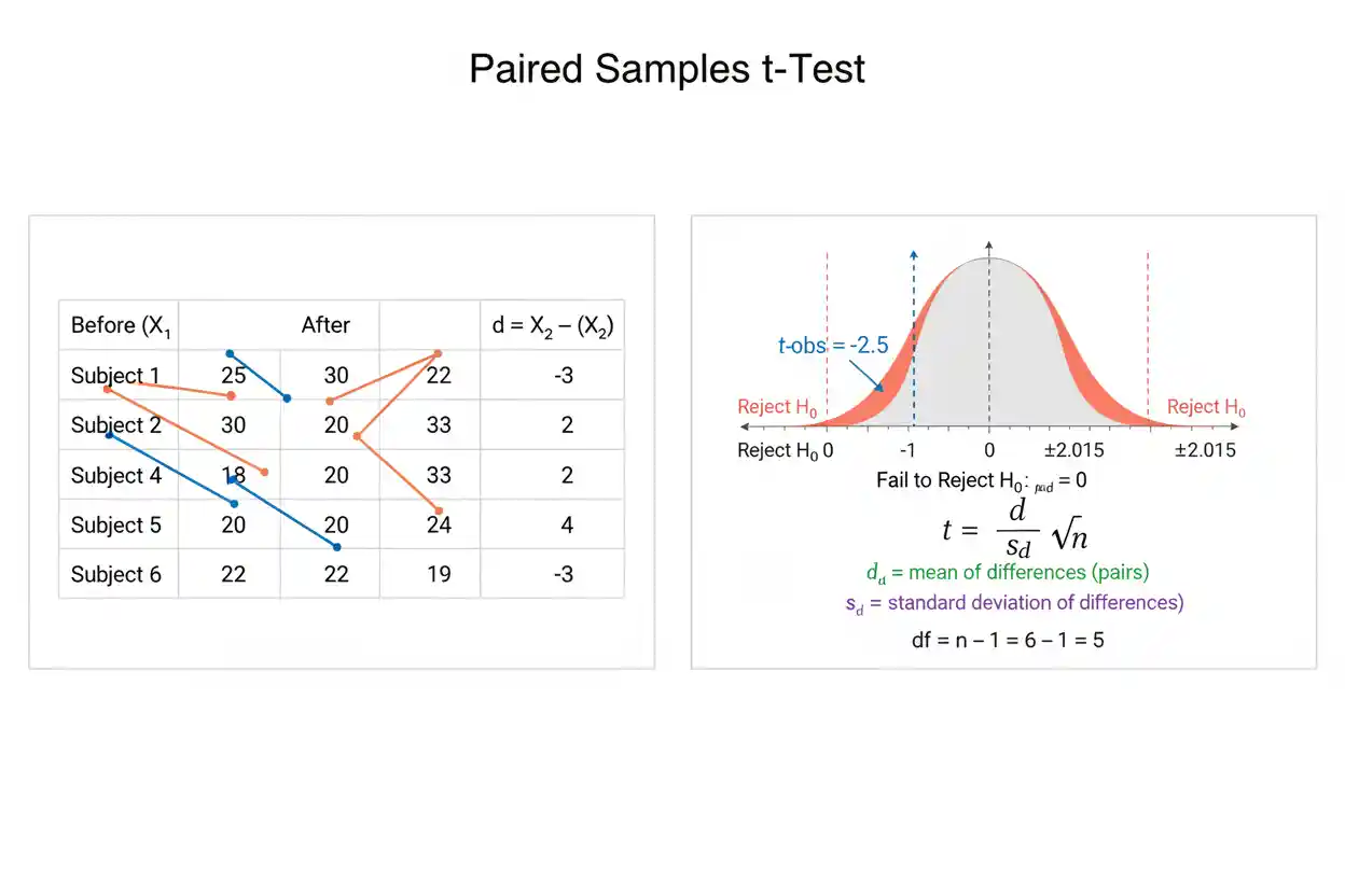

A paired t-test is an inferential statistical procedure used to evaluate the mean difference between two related measurements. The observations are paired because each value in one condition has a specific counterpart in the other condition, such as measurements taken from the same person before and after treatment, matched individuals selected according to relevant characteristics, or two measurements made on the same experimental unit. Rather than analyzing the two sets of scores as though they came from independent groups, the paired t-test calculates one difference for every pair and performs inference on the population mean of those differences. This transformation is the key to understanding the method: mathematically, the standard paired t-test is a one-sample t-test applied to the pairwise differences.
The test statistic compares the observed mean difference with a hypothesized mean difference, usually zero, and divides that discrepancy by the estimated standard error of the mean difference. Pairing can substantially improve precision when measurements within each pair are positively related because stable pair-specific characteristics are removed when differences are calculated. However, pairing must arise from the study design; two samples should not be declared paired merely because they contain the same number of observations. Correct use also requires the pairs themselves to provide appropriately independent information and requires the distribution of pairwise differences—not necessarily each original measurement distribution—to support the intended t-based inference.
The paired t-test is part of Statistics & Probability and the broader Inference & Regression framework. Its core intent is specific: testing the population mean of within-pair differences for two related quantitative measurements.
What Is a Paired T-Test?
Suppose each observational unit produces two measurements, Xᵢ and Yᵢ. For every pair, define a difference:
Dᵢ = Xᵢ − Yᵢ
The paired-data problem can now be reduced to one quantitative variable:
D₁, D₂, …, Dₙ
The parameter of interest is:
μD = population mean of the paired differences
A common null hypothesis is:
H₀: μD = 0
with a two-sided alternative:
H₁: μD ≠ 0
If μD = 0, there is no population mean difference according to the defined subtraction order. If μD is positive, X tends to exceed Y on average. If μD is negative, X tends to be lower than Y on average.
The standard paired t statistic is:
t = (D̄ − μD,0) / (sD / √n)
where D̄ is the sample mean difference, μD,0 is the hypothesized population mean difference, sD is the sample standard deviation of the differences, and n is the number of complete pairs.
When the null value is zero:
t = D̄ / (sD / √n)
This equation contains the entire basic logic of the paired t-test.
Paired T-Test Formula
The calculation begins with one difference for each pair:
Dᵢ = Xᵢ − Yᵢ
The sample mean of those differences is:
D̄ = ΣDᵢ / n
The sample standard deviation of the differences is:
sD = √[Σ(Dᵢ − D̄)² / (n − 1)]
The estimated standard error of the mean difference is:
SE(D̄) = sD / √n
The test statistic is then:
t = (D̄ − μD,0) / SE(D̄)
or equivalently:
t = (D̄ − μD,0) / (sD / √n)
For the common zero-difference null:
t = D̄ / (sD / √n)
The statistic measures how many estimated standard errors the observed mean difference lies from the value stated by H₀.
Degrees of Freedom
The ordinary paired t-test has:
df = n − 1
where n is the number of complete pairs.
If 20 participants each provide a before and after measurement:
n = 20
and:
df = 19
The sample size is 20 pairs, not 40 independent observations. Although the dataset contains 40 raw measurements, those observations are organized into 20 dependent pairs.
This distinction is essential. Treating all 40 values as independent would ignore the within-person relationship and use the wrong sampling model.
Why the Test Uses Differences
Consider a before-and-after study in which some participants naturally score much higher than others. If those person-specific baseline differences remain relatively stable, comparing the two sets of scores as independent groups introduces substantial variability that has little to do with the change being studied.
Pairwise subtraction removes much of that stable between-person variation.
Suppose Participant A scores 95 before treatment and 100 afterward, while Participant B scores 45 before and 50 afterward. Their overall score levels differ dramatically, but both changed by five points.
The paired differences capture:
+5 and +5
rather than treating 95, 100, 45, and 50 as unrelated measurements.
The paired t-test therefore focuses directly on change within matched units.
Worked Paired T-Test Example
Suppose 10 participants complete a performance assessment before and after a training program. Define each difference as:
D = After − Before
Assume the observed differences are:
| Participant | Difference D |
|---|---|
| 1 | 3 |
| 2 | 5 |
| 3 | 4 |
| 4 | 6 |
| 5 | 2 |
| 6 | 5 |
| 7 | 7 |
| 8 | 4 |
| 9 | 3 |
| 10 | 6 |
The research question is whether the population mean change differs from zero.
The hypotheses are:
H₀: μD = 0
H₁: μD ≠ 0
The sample contains:
n = 10 pairs
Step 1: Calculate the Mean Difference
Add the observed differences:
ΣDᵢ = 3 + 5 + 4 + 6 + 2 + 5 + 7 + 4 + 3 + 6
ΣDᵢ = 45
Therefore:
D̄ = 45 / 10
D̄ = 4.5
The sample shows an average increase of 4.5 points.
Because the differences were defined as After − Before, a positive value represents improvement according to the direction used in this example.
Step 2: Calculate the Standard Deviation of the Differences
The squared deviations from D̄ = 4.5 sum to:
Σ(Dᵢ − D̄)² = 22.5
The sample variance of the differences is:
sD² = 22.5 / (10 − 1)
sD² = 22.5 / 9
sD² = 2.5
Therefore:
sD = √2.5
sD ≈ 1.581
The pairwise changes vary by approximately 1.58 points around their sample mean.
Step 3: Calculate the Standard Error
The estimated standard error of the mean difference is:
SE(D̄) = sD / √n
Substituting the values:
SE(D̄) = 1.581 / √10
SE(D̄) ≈ 1.581 / 3.162
SE(D̄) ≈ 0.500
The sample mean difference is therefore estimated with a standard error of approximately half a point.
Step 4: Calculate the T Statistic
The null mean difference is:
μD,0 = 0
Therefore:
t = (4.5 − 0) / 0.5
t = 9
The degrees of freedom are:
df = 10 − 1
df = 9
The observed result is:
t(9) = 9.00
The sample mean difference lies nine estimated standard errors above the null value.
Step 5: Interpret the P-Value
For:
t = 9
with:
df = 9
the two-sided p-value is approximately:
p ≈ 0.0000085
or:
p < 0.001
The P-Value represents the probability, assuming H₀ and the paired t-test model are correct, of obtaining a t statistic at least as extreme as the observed statistic according to the two-sided test.
At:
α = 0.05
the result is far below the rejection threshold, so H₀ is rejected.
The sample provides strong statistical evidence that the population mean paired difference is not zero.
The observed mean improvement is 4.5 points. Whether a 4.5-point change is practically important requires interpretation on the performance scale and cannot be determined by the p-value alone.
Confidence Interval for the Mean Difference
A confidence interval is often more informative than a significance decision alone because it describes the estimated magnitude and precision of μD.
A paired t confidence interval has the form:
D̄ ± t* × sD / √n
For the worked example:
D̄ = 4.5
SE(D̄) = 0.5
df = 9
For a 95% confidence interval, the two-sided t critical value is approximately:
t* ≈ 2.262
The margin of error is:
2.262 × 0.5
1.131
Therefore:
Lower bound = 4.5 − 1.131
Lower bound ≈ 3.369
Upper bound = 4.5 + 1.131
Upper bound ≈ 5.631
The approximate 95% confidence interval is:
3.37 to 5.63
Zero lies well outside this interval, which is consistent with rejecting H₀: μD = 0 in the corresponding two-sided test.
What the Confidence Interval Means
The interval estimates the population mean paired difference rather than the range of differences expected for individual future participants.
A conventional frequentist 95% confidence interval does not mean there is a 95% posterior probability that the fixed μD lies between 3.37 and 5.63 after the data have been observed. Its coverage property concerns repeated use of the interval-producing procedure under its assumptions.
It should also not be confused with a Prediction Interval. A prediction interval for a future individual difference would need to account for the variability of individual differences as well as uncertainty in the estimated population mean, so it is typically wider than a confidence interval for μD.
The two intervals answer different questions: one concerns a population mean, while the other concerns a future observation.
Paired T-Test Is a One-Sample Test on Differences
The most useful conceptual simplification is:
paired t-test = one-sample t-test applied to Dᵢ
After calculating:
Dᵢ = Xᵢ − Yᵢ
the original two-variable paired problem becomes a one-variable mean problem.
The hypotheses become:
H₀: μD = μD,0
H₁: μD ≠ μD,0
and the test statistic is simply:
t = (D̄ − μD,0) / (sD / √n)
This equivalence explains why the degrees of freedom are n − 1 and why assumptions about normality apply primarily to the differences rather than independently to each original measurement.
What Counts as Paired Data?
Paired data arise when each observation in one condition has a meaningful, predetermined connection with exactly one observation in the other condition.
A common example is repeated measurement of the same person:
before treatment ↔ after treatment
Another is measurement of the same physical unit under two conditions:
machine under setting A ↔ same machine under setting B
Matched designs can also create pairs:
treated participant ↔ specifically matched control participant
The defining feature is the relationship between members of each pair.
Two unrelated samples do not become paired simply because they both contain 30 observations.
Before-and-After Studies
Before-and-after designs are among the clearest applications of the paired t-test. Each participant serves as their own comparison unit.
Suppose blood pressure, reaction time, productivity, or examination performance is measured before an intervention and again afterward.
For participant i:
Dᵢ = Afterᵢ − Beforeᵢ
The paired t-test evaluates whether the population mean of those changes differs from the null value.
The test does not automatically prove that the intervention caused the change. Without an appropriate control design, observed changes can also arise from time trends, regression to the mean, external events, measurement changes, practice effects, or other factors.
Pairing addresses statistical dependence; it does not by itself establish causal identification.
Matched Pairs
Not every paired design requires repeated measurement of exactly the same entity. Researchers may deliberately match two separate units according to variables expected to influence the outcome.
For example, each treated participant might be matched with a control participant of similar age, baseline score, and another relevant characteristic.
A difference is then calculated within each matched pair.
The quality of such a design depends on whether the matching strategy creates meaningful comparable pairs. Simply pairing observations arbitrarily does not provide the same benefit and can make the interpretation meaningless.
The statistical method should reflect the actual design rather than a convenient arrangement of spreadsheet rows.
Why Pairing Can Increase Precision
Pairing is especially useful when the two measurements within a pair are positively correlated.
Suppose people who score high before an intervention also tend to score high afterward. Much of the total variability in the raw scores reflects stable differences among people rather than variation in treatment response.
Subtracting within each participant removes much of that stable person-specific component.
The variance of a difference between two variables is:
Var(X − Y) = Var(X) + Var(Y) − 2Cov(X,Y)
If X and Y are positively correlated:
Cov(X,Y) > 0
the subtraction term reduces the variance of the paired differences.
A smaller sD produces a smaller standard error:
SE(D̄) = sD / √n
which can increase precision.
Pairing Does Not Always Improve Precision
Pairing is not automatically superior simply because it is available.
If measurements within pairs have little correlation, the reduction in variability may be limited. If pair formation is poor or arbitrary, the design may provide little advantage.
More importantly, a study should not create artificial pairings after data collection merely to search for a more favorable test statistic.
The pairing structure must be substantively justified by the design.
When observations genuinely come from unrelated groups, an independent-samples procedure rather than a paired test is appropriate.
Direction of the Difference Matters
The sign of the mean difference depends on how D is defined.
If:
D = After − Before
then:
D̄ > 0
indicates an average increase.
If the subtraction is reversed:
D = Before − After
the same data produce:
D̄ < 0
The absolute t statistic and two-sided p-value remain unchanged because both the numerator and its sign reverse consistently.
However, directional interpretation changes.
For one-sided tests especially, the difference convention should be defined before calculations are performed.
Two-Sided Paired T-Test
A two-sided paired t-test evaluates departures in either direction.
The hypotheses are:
H₀: μD = 0
H₁: μD ≠ 0
Evidence against H₀ can arise from either a sufficiently positive or sufficiently negative mean difference.
The rejection rule has the general form:
Reject H₀ if |t| > tcritical
where the critical value depends on α and:
df = n − 1
Two-sided testing is appropriate when increases and decreases are both relevant to the research question.
Right-Tailed Paired T-Test
Suppose D is defined as:
D = After − Before
and the research question asks specifically whether the intervention increases the outcome.
The hypotheses can be:
H₀: μD = 0
H₁: μD > 0
The rejection region lies in the upper tail of the t distribution.
A large positive t statistic provides evidence in the specified direction.
A large negative statistic does not support H₁, even though its magnitude may be substantial.
The directional alternative should be established independently of the observed data.
Left-Tailed Paired T-Test
Suppose lower values after an intervention represent the expected improvement and D remains defined as:
After − Before
The hypotheses might be:
H₀: μD = 0
H₁: μD < 0
A sufficiently negative t statistic provides evidence against H₀ in the hypothesized direction.
Again, changing the direction of the alternative after inspecting the result invalidates the intended one-sided error rate.
Testing a Nonzero Mean Difference
Although zero is the most common null value, the paired t-test can evaluate another specified difference.
Suppose an intervention is considered meaningfully improved only if the population mean increase equals a benchmark of 2 units.
A test could mathematically evaluate:
H₀: μD = 2
using:
t = (D̄ − 2) / (sD / √n)
The paired t-test is therefore not inherently limited to a null difference of zero.
However, questions about whether an effect exceeds a practically meaningful threshold may require carefully chosen directional or equivalence/noninferiority procedures rather than a simple point-null test, depending on the objective.
Assumptions of the Paired T-Test
The paired t-test requires a quantitative paired-difference variable for which the mean is meaningful. Each pair should represent a genuine repeated or matched structure, and different pairs should provide appropriately independent information. Exact classical small-sample inference assumes the population distribution of the pairwise differences is normal.
The normality condition applies to:
Dᵢ = Xᵢ − Yᵢ
not necessarily to X and Y separately.
The method is often reasonably robust to moderate departures from normality when the sample of independent pairs is sufficiently informative and the difference distribution is not dominated by severe skewness or extreme outliers. However, no universal sample-size threshold guarantees robustness.
The assumptions should be evaluated in relation to the differences and the sampling design rather than through mechanical rules.
Independence Is Between Pairs
Measurements inside each pair are expected to be related. That dependence is precisely why a paired method is being used.
The independence requirement concerns separate pairs.
For example, if 30 different participants each supply a before and after measurement, Participant 1’s pair should ideally provide information that is appropriately independent of Participant 2’s pair under the sampling model.
If participants are strongly clustered within families, teams, classrooms, or other structures, additional dependence may remain even after pairwise differencing.
The ordinary paired t-test does not automatically account for those higher-level dependencies.
Normality of the Differences
Suppose Before scores are strongly skewed and After scores are also strongly skewed. This does not automatically invalidate the paired t-test.
The relevant variable is:
D = After − Before
If the distribution of D is approximately normal or the mean difference has an adequately normal sampling distribution, t-based inference may still perform well.
Conversely, two individually normal-looking measurement distributions do not guarantee that the paired differences are well behaved.
Statistical diagnostics should therefore focus on the difference scores.
Outliers in the Differences
The sample mean and sample standard deviation are both sensitive to extreme observations. An unusual paired difference can therefore strongly affect the t statistic.
Suppose most participants change by 2 to 5 points, but one participant changes by 80 points. That value can shift D̄ and inflate sD simultaneously.
The observation should be investigated to determine whether it is:
a recording error, a measurement problem, a legitimate extreme response, or evidence that the mean is not an adequate summary of the change distribution.
A valid extreme observation should not be deleted merely because its removal produces a more favorable p-value.
Sample Size
The relevant sample size is the number of complete pairs:
n = number of D values
If 50 participants enter a before-and-after study but only 42 provide both measurements, the ordinary complete-pair analysis has:
n = 42
unless missing data are handled through another justified method.
The eight incomplete cases do not each contribute half a pair to the standard calculation.
Missing paired measurements can also introduce bias when missingness is related to the outcome or change process, so loss of pairs is not only a sample-size issue.
No Universal n = 30 Rule
There is no universal rule that a paired t-test becomes automatically valid at:
n = 30
A nearly symmetric difference distribution without extreme values may support good inference with fewer observations.
An extremely skewed or heavy-tailed difference distribution can require substantially more observations before a normal approximation for D̄ becomes adequate.
The appropriate sample size depends on the behavior of the differences, the degree of independence, the required inferential accuracy, and the study design.
Thirty is at most a rough teaching convention in some contexts, not a theorem.
Paired T-Test vs Independent T-Test
The difference between paired and independent tests is determined by the data structure.
Paired:
each observation in condition A has a specific counterpart in condition B
Independent:
observations in one group are unrelated to observations in the other group
Using an independent analysis on genuinely paired data ignores information about within-pair relationships and may reduce precision.
Using a paired analysis on unrelated groups creates artificial differences that have no natural interpretation.
The test should therefore be selected from the study design before considering which method gives a smaller p-value.
Paired T-Test vs One-Way ANOVA
The One-Way Anova is designed to evaluate equality among means of independent groups defined by one categorical factor under its standard formulation.
A paired t-test instead concerns two related conditions.
For example:
same 25 patients before and after treatment
is a paired design.
By contrast:
25 patients receiving Treatment A, 25 different patients receiving Treatment B, and 25 different patients receiving Treatment C
is an independent multi-group structure that may fit a one-way ANOVA question.
Repeated measurements across three or more conditions require methods designed for repeated or dependent observations rather than ordinary independent one-way ANOVA.
Paired T-Test vs One-Sample Z-Test
A paired t-test is fundamentally a mean test on the difference scores when the population standard deviation of those differences is unknown and estimated by sD.
The One-Sample Z-Test uses a known population standard deviation under its classical mean-testing formulation.
For paired differences, if the population standard deviation σD were genuinely known and the appropriate conditions held, a z statistic could conceptually be:
z = (D̄ − μD,0) / (σD / √n)
In ordinary applications, σD is generally unknown, so the t-based procedure using sD is the natural framework.
The distinction is based on how uncertainty in the difference distribution is handled rather than a simplistic small-sample-versus-large-sample rule.
Connection to an Intercept-Only Regression
After pairwise differences have been calculated, the paired t-test can also be represented as an intercept-only linear model:
Dᵢ = β₀ + εᵢ
The intercept represents the population mean difference:
β₀ = μD
Testing:
H₀: μD = 0
is therefore equivalent to testing:
H₀: β₀ = 0
in this simple model under corresponding assumptions.
This connection helps explain why t-based inference appears throughout linear modeling. The broader meaning and interpretation of a Regression Intercept extends beyond paired comparisons, while the paired t-test remains specifically focused on the mean of within-pair differences.
Effect Size for Paired Data
Statistical significance does not indicate how large the paired change is.
One standardized paired effect uses the standard deviation of the differences:
dᶻ = D̄ / sD
For the worked example:
D̄ = 4.5
sD ≈ 1.581
Therefore:
dᶻ = 4.5 / 1.581
dᶻ ≈ 2.85
This represents a very large standardized mean difference relative to the variability of the individual change scores in this constructed example.
Other standardized effect definitions exist for repeated-measures designs and can use different denominators. Therefore, the calculation method should be stated explicitly rather than reporting an unexplained “d.”
Relationship Between Paired d and t
For the version:
dᶻ = D̄ / sD
and the zero-null paired t statistic:
t = D̄ / (sD / √n)
the relationship is:
t = dᶻ√n
For the worked example:
dᶻ ≈ 2.846
and:
√10 ≈ 3.162
Therefore:
t ≈ 2.846 × 3.162
t ≈ 9
This relationship demonstrates why the t statistic incorporates both effect magnitude and sample size.
The standardized effect measures magnitude relative to variation in the differences. The t statistic additionally reflects how precisely that mean difference has been estimated.
Statistical Significance vs Practical Importance
Suppose a study of 50,000 paired observations finds an average change of:
D̄ = 0.05
with a tiny standard error.
The paired t-test may produce:
p < 0.001
yet a change of 0.05 units might be operationally meaningless.
Another study might estimate:
D̄ = 8
but contain only six highly variable pairs, resulting in substantial uncertainty and a nonsignificant p-value.
The first study has stronger statistical evidence against a zero mean difference. The second has the larger observed raw effect.
Neither conclusion alone determines which result matters more in practice.
Type I Error
A Type I error occurs when the test rejects:
H₀: μD = μD,0
even though that null condition is true.
If:
α = 0.05
the testing procedure is constructed so that, under H₀ and the required assumptions, its long-run probability of false rejection is 5%.
This does not mean that a particular significant result has a 5% probability of being false.
The probability refers to repeated use of the testing procedure under the null model.
Type II Error and Power
A Type II error occurs when the paired t-test fails to reject H₀ even though the population mean difference meaningfully departs from the null value.
Statistical power generally improves when the true mean difference becomes larger, the number of independent pairs increases, the standard deviation of the differences becomes smaller, or the significance threshold becomes less restrictive.
Strong positive within-pair correlation can indirectly improve power because it can reduce sD.
This is one reason a properly designed paired study can achieve more precision than an independent comparison using a similar number of observational units.
Failure to Reject Does Not Prove No Change
Suppose a paired study estimates:
D̄ = 3
but produces a 95% confidence interval of:
−4 to 10
The corresponding two-sided test will fail to reject a zero mean difference.
Yet the data remain compatible with meaningful decreases and meaningful increases.
The correct conclusion is not:
the intervention has no effect
but rather that the study does not estimate the mean change precisely enough to exclude zero.
If the research objective is to demonstrate that any difference is smaller than a predefined practically important margin, an equivalence analysis is more appropriate.
Missing Pairs
The ordinary paired calculation requires a difference for every included observational unit.
If a participant has a Before measurement but no After measurement, D cannot be calculated directly.
Discarding all incomplete pairs may be reasonable under some missing-data mechanisms but can create bias under others. For example, participants who experienced poor outcomes may be disproportionately likely to miss the follow-up measurement.
The paired t-test itself does not solve missing-data problems.
The mechanism and amount of missingness should therefore be considered before interpreting the resulting sample as representative.
Order Effects and Repeated Measurement
In studies where the same person experiences two conditions sequentially, the second measurement can be influenced by the first condition.
Potential effects include:
practice, fatigue, learning, carryover, adaptation, or time trends.
A paired t-test correctly accounts for the statistical pairing, but it does not eliminate these design effects.
For crossover or repeated-condition experiments, counterbalancing, washout periods, random condition order, or more specialized models may be required depending on the scientific question.
Statistical pairing and experimental control are separate issues.
Pairing Does Not Prove Causation
Suppose average performance rises significantly after a training program.
Even though before and after measurements come from the same participants, other explanations can remain:
participants may improve through practice, outside conditions may change, regression to the mean may occur, measurement procedures may differ, or unrelated time trends may influence the outcome.
A paired design removes stable between-participant differences but does not automatically create a valid counterfactual for what would have happened without the intervention.
Causal conclusions require an appropriate experimental or quasi-experimental design beyond the choice of statistical test.
Common Mistakes
A frequent mistake is treating two equal-sized independent samples as paired. Equal sample sizes do not create a pairing relationship.
Another mistake is testing the original Before and After distributions separately for normality while ignoring the distribution of the actual difference scores. The paired test operates on D.
Researchers also sometimes count 20 pairs as n = 40. For the paired t-test:
n = number of pairs
Another error is interpreting a significant result as evidence that every participant improved. A positive mean difference can coexist with some participants showing no change or movement in the opposite direction.
A nonsignificant result should not be interpreted as proof of no change, and a small p-value should not be interpreted as the probability that H₀ is true.
Finally, a paired t-test can establish evidence of a mean change without establishing that the change was caused by the intervention.
How to Perform a Paired T-Test
Begin by confirming that each measurement in one condition has a genuine counterpart in the other condition. Define the subtraction order clearly:
Dᵢ = Xᵢ − Yᵢ
Calculate all complete pairwise differences, then calculate:
D̄ = ΣDᵢ / n
and:
sD = √[Σ(Dᵢ − D̄)² / (n − 1)]
Calculate the standard error:
SE(D̄) = sD / √n
State the null hypothesis:
H₀: μD = μD,0
Then calculate:
t = (D̄ − μD,0) / (sD / √n)
with:
df = n − 1
Use the relevant t distribution to obtain a p-value or critical-value decision. Finally, interpret the result together with the mean difference, confidence interval, practical context, and quality of the pairing design.
How to Report a Paired T-Test
A useful report should include the direction used to define the differences, mean difference, t statistic, degrees of freedom, p-value, and preferably a confidence interval.
For the worked example:
Mean difference = 4.50
t(9) = 9.00
p < 0.001
95% CI ≈ 3.37 to 5.63
A contextual report could state that post-training scores were on average 4.5 points higher than pre-training scores, with strong statistical evidence that the population mean paired difference was greater than zero according to the two-sided paired t-test.
The substantive importance of 4.5 points should then be evaluated on the actual performance scale.
Frequently Asked Questions
What is a paired t-test?
A paired t-test evaluates the population mean difference between two related quantitative measurements by performing a one-sample t-test on the pairwise difference scores.
What is the paired t-test formula?
The standard formula is:
t = (D̄ − μD,0) / (sD / √n)
For a zero-difference null:
t = D̄ / (sD / √n)
How do you calculate paired differences?
Choose a consistent subtraction order:
Dᵢ = Xᵢ − Yᵢ
For before-and-after data, you might define:
Dᵢ = Afterᵢ − Beforeᵢ
What is the null hypothesis?
A common null is:
H₀: μD = 0
This states that the population mean paired difference is zero.
What does n mean in a paired t-test?
n is the number of complete pairs, not the number of individual raw measurements.
What are the degrees of freedom?
For n complete pairs:
df = n − 1
What is the standard error?
The estimated standard error of the mean difference is:
SE(D̄) = sD / √n
Is the paired t-test the same as a one-sample t-test?
Mathematically, yes after the pairwise differences have been calculated. The paired t-test is a one-sample t-test applied to D.
When should I use a paired t-test?
Use it when two quantitative measurements are genuinely related, such as before-and-after measurements from the same individuals or deliberately matched pairs.
Can I use a paired t-test for two independent groups of equal size?
No. Equal group sizes do not establish pairing. Each observation must have a meaningful counterpart.
Does the test require normal data?
Exact classical small-sample inference assumes the population distribution of the pairwise differences is normal. The original X and Y variables do not each need to be normally distributed merely for the differences to be analyzed.
Which distribution should be checked for normality?
The pairwise differences:
Dᵢ
are the relevant distribution.
Does n = 30 guarantee the test is valid?
No. There is no universal n = 30 rule. Robustness depends on the shape and tail behavior of the difference distribution, independence, outliers, and required accuracy.
Can the paired t-test be one-sided?
Yes. Directional alternatives such as:
H₁: μD > 0
or:
H₁: μD < 0
can be used when justified in advance.
What does a positive t statistic mean?
Its direction depends on how the differences were defined. If D = After − Before, a positive t generally reflects an average increase.
Does a significant paired t-test mean everyone improved?
No. It concerns the population mean difference. Individual pairs can move in different directions.
Does a significant paired t-test prove treatment caused the change?
No. Causal interpretation depends on study design and control of alternative explanations.
What does a nonsignificant paired t-test mean?
It means the sample does not provide sufficiently strong evidence against the stated mean-difference null at the chosen threshold. It does not prove that the population mean difference is exactly zero.
Why can pairing increase power?
When measurements within pairs are positively correlated, subtracting them can remove stable pair-level variability and reduce the standard deviation of the differences.
What is the difference between a confidence interval and prediction interval here?
A confidence interval estimates the population mean difference. A prediction interval concerns the value of a future individual difference and is generally wider because individual variation must also be included.
Should an effect size be reported?
When magnitude matters, yes. The mean difference in original units and an appropriate standardized paired effect can complement the p-value and confidence interval.
Key Takeaway
The paired t-test evaluates the population mean difference between two genuinely related measurements. Its defining step is to convert every pair into a single difference:
Dᵢ = Xᵢ − Yᵢ
The sample mean difference is:
D̄ = ΣDᵢ / n
and its estimated standard error is:
SE(D̄) = sD / √n
The resulting test statistic is:
t = (D̄ − μD,0) / (sD / √n)
with:
df = n − 1
For the common zero-difference hypothesis:
H₀: μD = 0
the method asks whether the observed average within-pair difference is large relative to its sampling uncertainty. Pairing can improve precision by removing stable variation between matched units, but only when the pairs are genuinely defined by the study design. The important assumptions concern independence between pairs and the behavior of the pairwise differences, not independence of the two observations within each pair. A statistically significant result provides evidence that the population mean difference departs from its null value; it does not prove that every pair changed, that the effect is practically important, or that the measured change was caused by the intervention.



