
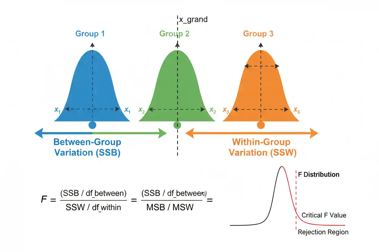

One-way ANOVA, short for one-way analysis of variance, is an inferential statistical procedure used to test whether the population means of several independent groups can reasonably be treated as equal. Instead of conducting a separate comparison for every pair of groups, one-way ANOVA evaluates all group means simultaneously through a single F statistic. The method works by comparing variation between the group means with variation observed among individuals within the groups. If the group means are genuinely similar, between-group variation should generally be comparable with the background variation found within groups.
If the group means are much farther apart than ordinary within-group variability would predict, the resulting F statistic becomes large and provides evidence against the null hypothesis of equal population means. A significant result indicates that not all population means are equal, but it does not by itself identify exactly which groups differ. One-way ANOVA also does not establish practical importance merely because the result is statistically significant. Appropriate interpretation requires attention to independent observations, group distributions, variance behavior, sample size, outliers, effect magnitude, and any follow-up comparisons required by the research question.
One-way ANOVA belongs to Statistics & Probability and forms an important part of Inference & Regression. Its core purpose is specific: testing equality among the means of independent groups defined by one categorical factor.
What Is One-Way ANOVA?
One-way ANOVA tests whether the means of two or more independent populations are equal when observations are grouped according to one categorical explanatory variable, commonly called a factor.
Suppose a researcher wants to compare average performance under three teaching methods. The factor is teaching method, and it has three levels:
- Method A
- Method B
- Method C
The response variable is a quantitative performance score.
The population means can be represented as:
μ₁, μ₂, μ₃
The Null Hypothesis is:
H₀: μ₁ = μ₂ = μ₃
More generally, for k groups:
H₀: μ₁ = μ₂ = … = μₖ
The alternative is:
H₁: not all population means are equal
This wording matters. The alternative does not state that every mean differs from every other mean. Rejecting H₀ requires only that at least one population mean differs from at least one other population mean.
Why Is It Called Analysis of Variance?
The procedure tests means, yet its name refers to variance because the evidence about mean differences is obtained by decomposing variability.
One-way ANOVA separates total variability in the response into two broad components:
variation between groups
and:
variation within groups
Between-group variation measures how far the individual group means lie from the grand mean. Within-group variation measures how far individual observations lie from their own group means.
If H₀ is reasonable, the group means should not usually be separated by much more than ordinary sampling variation would predict. The between-group and within-group variance estimates should therefore be broadly comparable.
When genuine population mean differences exist, the group means tend to be farther apart, increasing the between-group component while the within-group component continues to represent background variability.
The ratio between those components becomes the F statistic.
The One-Way ANOVA Model
A standard conceptual model can be written as:
Yᵢⱼ = μ + αⱼ + εᵢⱼ
where:
- Yᵢⱼ = observation i in group j
- μ = overall mean component
- αⱼ = effect associated with group j
- εᵢⱼ = random deviation within the group
An equivalent mean-based view is that each group has its own population mean μⱼ and observations vary around that mean.
The null hypothesis of equal group means corresponds to the absence of systematic differences among the group mean components.
For an ordinary fixed-effects one-way comparison:
H₀: μ₁ = μ₂ = … = μₖ
The model provides a framework for dividing the observed variability into variation associated with group membership and residual variation within groups.
The Grand Mean
The grand mean is the mean of all observations across all groups:
x̄grand = Σxᵢ / N
where N is the total number of observations.
If group sizes are equal, the grand mean also equals the simple average of the group means.
If group sizes differ, the grand mean is a weighted average of the group means because larger groups contribute more observations.
Suppose three groups have means:
x̄₁ = 10
x̄₂ = 15
x̄₃ = 20
If each group contains the same number of observations:
x̄grand = (10 + 15 + 20) / 3
x̄grand = 15
If the group sizes are unequal, simply averaging those three means may not produce the actual grand mean.
Total Sum of Squares
The total sum of squares measures total observed variation around the grand mean:
SST = Σ(xᵢⱼ − x̄grand)²
It answers the question:
How much do all individual observations vary around the overall mean?
In the standard one-way ANOVA decomposition:
SST = SSB + SSW
where:
- SSB = between-group sum of squares
- SSW = within-group sum of squares
Some sources use different abbreviations such as SSbetween, SSwithin, SSE, or SSTR. The notation may differ, but the statistical decomposition is the same when the quantities are defined consistently.
Between-Group Sum of Squares
The between-group sum of squares measures how far the group means lie from the grand mean while accounting for group sizes.
Its formula is:
SSB = Σnⱼ(x̄ⱼ − x̄grand)²
where:
- nⱼ = sample size of group j
- x̄ⱼ = sample mean of group j
- x̄grand = grand mean
If group means are close together, SSB will tend to be relatively small.
If group means are widely separated, SSB becomes larger.
The multiplication by nⱼ matters because a difference in a group mean based on many observations contributes differently from the same difference based on very few observations.
Within-Group Sum of Squares
The within-group sum of squares measures variation of individual observations around their own group means:
SSW = ΣΣ(xᵢⱼ − x̄ⱼ)²
This component reflects the background variation that remains after group membership has been accounted for.
Suppose every group has observations tightly concentrated near its own mean. SSW will be relatively small.
If individual observations vary greatly within each group, SSW will be larger.
The ANOVA F statistic evaluates group separation relative to this within-group variability. Therefore, the same difference between group means can produce very different F statistics depending on how noisy the observations are within groups.
The ANOVA Decomposition
For the ordinary one-way ANOVA:
SST = SSB + SSW
This equation partitions total observed variation into:
total variation = between-group variation + within-group variation
The relationship is central to the logic of ANOVA.
If group membership explains little about the response, most variability remains within groups and SSB represents only a small share of SST.
If the groups have substantially different means, more of the total variability is associated with differences among group means.
However, a large share of explained variation is not itself enough to establish statistical significance. Degrees of freedom and sampling variability must also be incorporated.
Degrees of Freedom
Suppose there are:
k groups
and:
N total observations
The between-group degrees of freedom are:
dfbetween = k − 1
The within-group degrees of freedom are:
dfwithin = N − k
The total degrees of freedom are:
dftotal = N − 1
These satisfy:
dftotal = dfbetween + dfwithin
because:
N − 1 = (k − 1) + (N − k)
Degrees of freedom are needed to convert sums of squares into mean squares, which provide variance-like quantities suitable for constructing the F statistic.
Mean Square Between Groups
The mean square between groups is:
MSB = SSB / (k − 1)
This converts the between-group sum of squares into a variance-like quantity by dividing by its degrees of freedom.
A large MSB means the group means display substantial variation around the grand mean after accounting for the number of independent group contrasts available.
Under H₀ and the classical assumptions, MSB and the within-group mean square estimate the same underlying error variance in expectation.
Under alternatives with genuinely different population means, MSB tends to become larger.
Mean Square Within Groups
The mean square within groups is:
MSW = SSW / (N − k)
MSW estimates the ordinary within-group error variance under the standard equal-variance ANOVA model.
It summarizes the background variability against which differences among the group means are compared.
A smaller MSW means individual observations are relatively tightly clustered around their group means.
A larger MSW means substantial variability exists even among observations belonging to the same group.
This denominator is fundamental to the F ratio.
One-Way ANOVA F Statistic
The one-way ANOVA test statistic is:
F = MSB / MSW
or:
F = [SSB / (k − 1)] / [SSW / (N − k)]
The statistic is nonnegative:
F ≥ 0
because both mean squares are based on sums of squared deviations.
When the null hypothesis is true, MSB and MSW should generally estimate comparable variance quantities, so F is often around 1, although random sampling variation can produce values above or below 1.
When group means are substantially different relative to within-group variability, MSB becomes large relative to MSW and F increases.
The one-way ANOVA test therefore uses the upper tail of an F distribution.
Worked One-Way ANOVA Example
Suppose three independent groups contain the following observations:
| Group A | Group B | Group C |
|---|---|---|
| 8 | 5 | 10 |
| 9 | 4 | 9 |
| 6 | 6 | 11 |
| 7 | 5 | 10 |
Each group contains:
n = 4
so:
N = 12
The group means are:
x̄A = (8 + 9 + 6 + 7) / 4 = 7.5
x̄B = (5 + 4 + 6 + 5) / 4 = 5
x̄C = (10 + 9 + 11 + 10) / 4 = 10
The total of all observations is:
30 + 20 + 40 = 90
Therefore, the grand mean is:
x̄grand = 90 / 12
x̄grand = 7.5
The question is whether the three population means can reasonably be treated as equal.
Step 1: State the Hypotheses
The null hypothesis is:
H₀: μA = μB = μC
The alternative is:
H₁: not all three population means are equal
Notice that H₁ does not claim:
μA ≠ μB ≠ μC
It only requires some departure from complete equality.
Step 2: Calculate the Between-Group Sum of Squares
Use:
SSB = Σnⱼ(x̄ⱼ − x̄grand)²
For Group A:
4(7.5 − 7.5)² = 0
For Group B:
4(5 − 7.5)²
= 4(−2.5)²
= 4(6.25)
= 25
For Group C:
4(10 − 7.5)²
= 4(2.5)²
= 25
Therefore:
SSB = 0 + 25 + 25
SSB = 50
Step 3: Calculate the Within-Group Sum of Squares
For Group A, whose mean is 7.5:
(8 − 7.5)² + (9 − 7.5)² + (6 − 7.5)² + (7 − 7.5)²
= 0.25 + 2.25 + 2.25 + 0.25
= 5
For Group B, whose mean is 5:
(5 − 5)² + (4 − 5)² + (6 − 5)² + (5 − 5)²
= 0 + 1 + 1 + 0
= 2
For Group C, whose mean is 10:
(10 − 10)² + (9 − 10)² + (11 − 10)² + (10 − 10)²
= 0 + 1 + 1 + 0
= 2
Therefore:
SSW = 5 + 2 + 2
SSW = 9
Step 4: Calculate Degrees of Freedom
There are:
k = 3 groups
so:
dfbetween = k − 1
dfbetween = 2
There are:
N = 12 observations
so:
dfwithin = N − k
dfwithin = 12 − 3
dfwithin = 9
The total degrees of freedom are:
dftotal = N − 1
dftotal = 11
and:
2 + 9 = 11
as required.
Step 5: Calculate the Mean Squares
The between-group mean square is:
MSB = SSB / dfbetween
MSB = 50 / 2
MSB = 25
The within-group mean square is:
MSW = SSW / dfwithin
MSW = 9 / 9
MSW = 1
Step 6: Calculate the F Statistic
Now calculate:
F = MSB / MSW
F = 25 / 1
F = 25
The test statistic is therefore:
F(2, 9) = 25
The first degrees-of-freedom value corresponds to the numerator, and the second corresponds to the denominator.
Step 7: Calculate the P-Value
For:
F = 25
with:
df₁ = 2
and:
df₂ = 9
the upper-tail probability is approximately:
p ≈ 0.00021
The P-Value is extremely small.
If:
α = 0.05
then:
p < α
so H₀ is rejected.
The data provide strong statistical evidence that the three population means are not all equal.
The conclusion is not that every pair of means necessarily differs. The overall ANOVA only establishes evidence against complete equality.
ANOVA Table
The worked example can be summarized in an ANOVA table:
| Source | Sum of Squares | df | Mean Square | F |
|---|---|---|---|---|
| Between groups | 50 | 2 | 25 | 25 |
| Within groups | 9 | 9 | 1 | |
| Total | 59 | 11 |
The total sum of squares is:
SST = SSB + SSW
SST = 50 + 9
SST = 59
The table condenses the decomposition and F calculation into a standard format.
What Does a Significant One-Way ANOVA Mean?
A significant result means the sample provides evidence against the hypothesis that all population group means are equal.
For three groups:
reject H₀: μ₁ = μ₂ = μ₃
means the data support the conclusion that at least one population mean differs.
It does not tell you automatically whether:
μ₁ differs from μ₂
μ₁ differs from μ₃
μ₂ differs from μ₃
or all three differ.
Those are more specific pairwise or contrast questions and require appropriate follow-up procedures.
The overall ANOVA should therefore be interpreted as an omnibus test.
What Does a Nonsignificant ANOVA Mean?
Suppose:
p = 0.32
with:
α = 0.05
The appropriate decision is:
fail to reject H₀
This means the sample does not provide sufficiently strong evidence that the population means differ.
It does not prove:
μ₁ = μ₂ = … = μₖ
A nonsignificant result can occur because the population means are genuinely similar, the differences are modest, within-group variability is large, sample sizes are small, or the study has limited statistical power.
Failure to reject equality is not proof of exact equality.
Why Not Run Several T-Tests?
Suppose four independent groups are compared. There are six possible pairwise comparisons.
If each comparison is conducted independently at:
α = 0.05
the overall probability of making at least one false-positive conclusion across the family can exceed 5%.
One-way ANOVA provides a single omnibus test of the global hypothesis:
H₀: all population means are equal
before more detailed comparisons are considered.
The procedure therefore addresses a multi-group question in a coherent inferential framework rather than treating every pair as an isolated experiment.
The One-Sample T-Test serves a different purpose: comparing one population mean with a fixed benchmark. It is not a substitute for a multi-group ANOVA.
One-Way ANOVA With Two Groups
Mathematically, one-way ANOVA can be performed with only two independent groups.
Under the standard equal-variance two-group setting, the ANOVA F statistic and corresponding two-sample t statistic are related by:
F = t²
when both tests represent the same two-sided comparison under compatible assumptions.
However, ANOVA becomes especially useful when three or more independent group means are being considered simultaneously.
The one-way ANOVA framework also generalizes naturally to partitioning variation across more than two groups.
One-Way ANOVA vs One-Sample T-Test
A One-Sample T-Test evaluates a question such as:
H₀: μ = 50
There is one population mean and one fixed reference value.
One-way ANOVA evaluates:
H₀: μ₁ = μ₂ = … = μₖ
There are multiple independent populations or groups whose means are compared with one another.
These tests therefore address different inferential structures even though both ultimately involve mean comparisons.
One-Way ANOVA vs One-Sample Z-Test
The One-Sample Z-Test tests one population mean against a specified benchmark under known-population-standard-deviation conditions.
For example:
H₀: μ = 100
One-way ANOVA instead compares several group means and uses an F statistic based on between-group and within-group variance estimates.
The two procedures have different null hypotheses, statistics, degrees of freedom, and reference distributions.
The fact that both belong to mean-based inference does not make them interchangeable.
Independent Groups vs Paired Data
Standard one-way ANOVA assumes the groups contain appropriately independent observational units.
Suppose three treatments are assigned to three different sets of participants. That structure can fit an independent-groups one-way ANOVA when the other conditions are appropriate.
If the same individuals are measured repeatedly under several conditions, however, the measurements within a person are dependent. Ordinary independent-groups ANOVA does not model that repeated-measures structure correctly.
Likewise, if there are exactly two related measurements per subject, the Paired T-Test owns that specific two-condition paired comparison.
The design determines the method. Counting the number of group columns alone is not enough.
Assumptions of One-Way ANOVA
The classical one-way ANOVA model relies on several important assumptions.
The outcome should be quantitative and meaningful to summarize using means. The observations should provide appropriately independent information. Within each population or model-defined group, the residual distribution should be sufficiently compatible with the inference method, especially in small samples. The standard pooled-variance ANOVA also assumes a common population variance across groups.
These assumptions concern the model and sampling process rather than arbitrary requirements that every histogram look perfectly normal.
The consequences of assumption violations depend on their severity, sample sizes, balance among groups, and the inferential objective.
Independence
Independence is among the most important assumptions.
If one person’s response appears multiple times and each row is treated as an independent person, the nominal sample size can greatly exaggerate the amount of independent information available.
Other examples of dependence include:
- students within classrooms
- patients within hospitals
- employees within teams
- repeated measurements
- related family members
- time-dependent observations
Ordinary one-way ANOVA does not automatically adjust for those structures.
A large dataset with dependence can still yield misleadingly small standard errors and p-values if the dependence is ignored.
Normality
Exact classical F inference is associated with normally distributed errors within groups under the standard model.
However, one-way ANOVA can be reasonably robust to moderate departures from normality in many settings, particularly with balanced designs and adequate sample sizes.
Normality should not be evaluated solely through whether individual observations form visually perfect bell curves.
More serious concerns arise with:
- severe skewness
- heavy tails
- extreme outliers
- very small groups
- strong imbalance combined with other violations
The practical impact depends on the complete design rather than one simplistic normality rule.
Equal Variances
The standard pooled one-way ANOVA assumes:
σ₁² = σ₂² = … = σₖ²
That is, the population variance is assumed to be the same across groups.
This common variance is estimated by the within-group mean square:
MSW
If group variances differ substantially, especially when group sample sizes are also unequal, the ordinary F procedure can behave poorly.
Unequal variances should therefore be assessed in relation to group sizes and the substantive data structure rather than ignored because the group means are the primary target.
Alternative ANOVA procedures designed for unequal variances may be appropriate when the equal-variance assumption is not reasonable.
Balanced vs Unbalanced Groups
A balanced one-way design has equal group sample sizes:
n₁ = n₂ = … = nₖ
Balanced designs often make the classical ANOVA more robust to moderate variance differences and simplify interpretation.
An unbalanced design has unequal group sizes.
Unequal sample sizes are not automatically invalid, but they can make variance heterogeneity more consequential. A small high-variance group combined with a large low-variance group can affect the operating characteristics of the ordinary pooled F test differently from other imbalance patterns.
The sample-size structure should therefore be considered when evaluating model assumptions.
Outliers
ANOVA is based on means, variances, and squared deviations, all of which are sensitive to extreme observations.
An extreme value can:
- shift a group mean
- inflate within-group variance
- alter the grand mean
- change SSB
- change SSW
- substantially modify the F statistic
An outlier should be investigated rather than removed automatically.
If it represents a data-entry error, correction may be warranted. If it is a legitimate observation, removing it merely because it changes statistical significance is inappropriate.
Extreme values can also indicate that a mean-based Gaussian model is not a good representation of the data.
Sample Size Does Not Fix Every Problem
Increasing sample size can improve precision and make large-sample approximations more useful, but it does not solve every design or modeling problem.
A very large sample cannot repair:
- severe selection bias
- incorrect independence assumptions
- wrong group definitions
- systematic measurement error
- an inappropriate causal interpretation
Large samples can actually make tiny model deviations highly statistically detectable.
Statistical significance therefore becomes easier to achieve as information grows, while practical interpretation remains a separate question.
Effect of Within-Group Variability
Suppose two studies have identical group means:
10, 15, and 20
In Study A, observations within each group vary only slightly around those means.
In Study B, observations range extremely widely.
The between-group difference is numerically the same, but Study A will generally produce a larger F statistic because:
MSW is smaller
The F ratio explicitly compares group separation with background variability:
F = MSB / MSW
This is why raw differences between group means cannot be interpreted independently of within-group variation.
Effect of Sample Size on the F Test
Larger samples allow group means to be estimated more precisely.
Consequently, modest population differences can become statistically detectable when many independent observations are available.
A small study might fail to reject H₀ even when the observed group means appear meaningfully different because within-group uncertainty is large.
A huge study may reject H₀ for very small mean differences.
This reinforces the distinction between statistical significance and substantive magnitude.
Statistical Significance vs Practical Importance
Suppose three groups have population-like sample means of:
100.0
100.2
100.4
With an enormous sample and very small measurement variability, ANOVA could produce an extremely small p-value.
The statistical result would indicate strong evidence that the means are not exactly equal.
Yet a maximum difference of:
0.4 units
might have no practical consequence.
Conversely, differences of several meaningful units can remain statistically uncertain in a small noisy study.
A complete interpretation should therefore report both statistical evidence and effect magnitude.
Effect Size in One-Way ANOVA
One simple descriptive measure associated with the ANOVA decomposition is eta squared:
η² = SSB / SST
It describes the proportion of observed total sum-of-squares variation associated with between-group differences in the sample.
Using the worked example:
SSB = 50
SST = 59
so:
η² = 50 / 59
η² ≈ 0.847
Approximately 84.7% of the observed sum-of-squares variation is associated with differences among the group means in this small constructed example.
This should not be interpreted as proving that group membership causally explains 84.7% of the outcome. Causal interpretation requires an appropriate design.
The magnitude estimate should also be treated as a sample statistic rather than an exact population value.
ANOVA Does Not Prove Causation
A significant F test demonstrates evidence of differences among population means under the model and sampling assumptions. It does not automatically establish why those means differ.
Suppose an observational study compares average income across three education categories and obtains a significant ANOVA.
The difference could reflect education, age, occupation, location, family background, selection processes, or many other factors.
Group membership and outcome may be associated without a simple causal relationship.
Randomized experiments can strengthen causal interpretation when treatment assignment is genuinely randomized and the design is otherwise sound, but ANOVA itself is a statistical comparison tool rather than a causal guarantee.
What Happens After a Significant ANOVA?
A significant omnibus result establishes that complete equality of the population means is inconsistent with the data at the selected threshold.
The next question may be more specific:
Which groups differ?
That question can be addressed with planned contrasts or appropriate post-hoc comparisons depending on the study design and research objectives.
Those follow-up procedures need to account for the fact that multiple comparisons can increase false-positive risk.
The overall F test should not be misreported as though it already identified every pairwise difference.
Why Post-Hoc Comparisons Need Care
Suppose five groups are present. There are:
5 × 4 / 2 = 10
possible pairwise comparisons.
Testing all 10 independently at α = 0.05 can produce a familywise false-positive probability substantially larger than 0.05.
Post-hoc procedures can adjust comparison thresholds or use simultaneous inference to control relevant error rates.
The appropriate method depends on whether comparisons were planned, how many are performed, whether variances are equal, and what inferential error criterion matters.
For the core one-way ANOVA result, the main conclusion remains the omnibus statement about equality of means.
ANOVA and the P-Value
The P-Value for one-way ANOVA is an upper-tail probability from the relevant F distribution:
p-value = P(Fdf₁,df₂ ≥ Fobserved | H₀)
where:
df₁ = k − 1
and:
df₂ = N − k
A small p-value means an F statistic at least as large as the observed one would be unusual under the complete equal-means null model.
It does not mean:
P(H₀ is true) = p
Nor does it measure the magnitude of the differences among means.
The p-value addresses compatibility with H₀; effect estimates address magnitude.
Why the F Test Is Right-Tailed
The F statistic is:
F = MSB / MSW
Both numerator and denominator are nonnegative.
Evidence against H₀ occurs when between-group variation is unusually large relative to within-group variation, producing a large F ratio.
Therefore, the rejection region lies in the upper tail.
An F value close to zero is not evidence of dramatically unequal group means. It indicates that between-group mean-square variation is small relative to within-group variation.
The one-way ANOVA test therefore does not use symmetric ±F critical values.
Can F Be Less Than 1?
Yes.
If:
MSB < MSW
then:
F < 1
For example:
MSB = 4
MSW = 8
gives:
F = 0.5
This means the observed group-mean variability is smaller than the estimated within-group variability.
Because evidence against the equal-means null lies in the upper tail, an F statistic below 1 ordinarily does not support rejection in the standard one-way ANOVA.
The statistic does not need to be at least 1.
Can F Equal 1?
Yes.
If:
MSB = MSW
then:
F = 1
This represents equal estimated between-group and within-group mean-square quantities.
Under the null hypothesis, an F statistic around 1 is conceptually unsurprising because both mean squares estimate the same error variance under the classical model.
Random samples can still produce values either above or below 1.
Common Mistakes
A frequent mistake is interpreting a significant ANOVA as proof that every group differs from every other group. The test establishes only that not all population means are equal.
Another mistake is performing many unadjusted pairwise comparisons instead of recognizing the multi-group inferential structure.
Researchers also sometimes ignore independence because every measurement appears on a separate spreadsheet row. Separate rows do not guarantee independent observations.
A fourth error is assuming equal sample sizes are required. ANOVA can accommodate unequal sample sizes, although imbalance makes some assumption violations more consequential.
Another misconception is that a nonsignificant result proves the means are equal. Failure to reject does not establish exact equality.
It is also incorrect to interpret the p-value as the probability H₀ is true or a statistically significant result as automatic evidence of practical importance.
Finally, ANOVA does not establish causation simply because group means differ.
How to Perform a One-Way ANOVA
Begin with one quantitative outcome and one categorical grouping variable representing independent groups.
State:
H₀: μ₁ = μ₂ = … = μₖ
and:
H₁: not all μⱼ are equal
Calculate each group mean and the grand mean.
Then calculate:
SSB = Σnⱼ(x̄ⱼ − x̄grand)²
and:
SSW = ΣΣ(xᵢⱼ − x̄ⱼ)²
Determine the degrees of freedom:
dfbetween = k − 1
dfwithin = N − k
Calculate:
MSB = SSB / (k − 1)
MSW = SSW / (N − k)
Then:
F = MSB / MSW
Use the F distribution with the appropriate numerator and denominator degrees of freedom to calculate the p-value or critical-value decision.
Finally, interpret the overall result without claiming pairwise differences the omnibus test did not establish.
How to Report a One-Way ANOVA
A concise result normally reports:
- the groups or factor
- the F statistic
- numerator degrees of freedom
- denominator degrees of freedom
- p-value
- relevant descriptive or effect-size information
For the worked example:
F(2, 9) = 25.00, p ≈ 0.00021
A clear interpretation is that the sample provides strong evidence that the three population means are not all equal.
The observed group means were:
7.5, 5.0, and 10.0
which provides important context for the direction and magnitude of the differences.
If specific pairwise claims are required, those should come from an appropriate follow-up analysis rather than being inferred automatically from the omnibus F statistic.
Frequently Asked Questions
What is one-way ANOVA?
One-way ANOVA is a statistical test used to evaluate whether the population means of independent groups defined by one categorical factor are all equal.
What does ANOVA stand for?
ANOVA stands for:
analysis of variance
It tests mean differences by comparing between-group and within-group variability.
What is the null hypothesis in one-way ANOVA?
For k groups:
H₀: μ₁ = μ₂ = … = μₖ
What is the alternative hypothesis?
The alternative is:
H₁: not all population means are equal
This means at least one mean differs, not necessarily every mean.
What is the formula for the F statistic?
The one-way ANOVA statistic is:
F = MSB / MSW
How is MSB calculated?
MSB = SSB / (k − 1)
where SSB is the between-group sum of squares.
How is MSW calculated?
MSW = SSW / (N − k)
where SSW is the within-group sum of squares.
What is the between-group sum of squares?
SSB = Σnⱼ(x̄ⱼ − x̄grand)²
It measures variation of group means around the grand mean.
What is the within-group sum of squares?
SSW = ΣΣ(xᵢⱼ − x̄ⱼ)²
It measures variation of individual observations around their own group means.
What are the degrees of freedom?
For k groups and N observations:
dfbetween = k − 1
dfwithin = N − k
What does a large F statistic mean?
A large F means between-group variability is large relative to within-group variability, which can provide evidence against equal population means.
Can F be less than 1?
Yes. F is nonnegative but can be below 1 when MSB is smaller than MSW.
Does significant ANOVA mean every group is different?
No. It means not all population means are equal. Additional comparisons are required to support specific pairwise claims.
What does a nonsignificant ANOVA mean?
It means the sample does not provide enough evidence to reject the equal-means null hypothesis at the selected significance level. It does not prove exact equality.
Can ANOVA compare only two groups?
Yes. One-way ANOVA can mathematically compare two independent groups, although two-group procedures may provide a more direct presentation for that specific case.
What is the difference between one-way ANOVA and a one-sample t-test?
A one-sample t-test compares one population mean with a fixed reference value. One-way ANOVA compares means across independent groups.
What is the difference between one-way ANOVA and paired t-test?
Standard one-way ANOVA assumes independent groups. A paired t-test is designed for two related measurements or matched observations.
Does ANOVA require equal sample sizes?
No. Unequal sample sizes are allowed, although imbalance can make variance heterogeneity and other assumption violations more important.
Does ANOVA require equal variances?
The standard pooled one-way ANOVA assumes a common population variance across groups. Alternative procedures can be preferable when this assumption is not reasonable.
Does ANOVA prove causation?
No. Mean differences demonstrate association with group membership. Causal interpretation depends on the study design and additional assumptions.
Should effect size be reported with ANOVA?
Usually, yes when magnitude matters. The F test addresses statistical evidence, while an effect-size measure helps describe how large the group-related differences are.
Key Takeaway
One-way ANOVA tests whether several independent population means can reasonably be treated as equal:
H₀: μ₁ = μ₂ = … = μₖ
The method divides observed variability into between-group and within-group components:
SST = SSB + SSW
with:
SSB = Σnⱼ(x̄ⱼ − x̄grand)²
and:
SSW = ΣΣ(xᵢⱼ − x̄ⱼ)²
Those quantities are converted into mean squares:
MSB = SSB / (k − 1)
MSW = SSW / (N − k)
and compared using:
F = MSB / MSW
A sufficiently large F statistic provides evidence that the population means are not all equal. It does not identify every pair that differs, establish practical importance, or prove causation. Reliable interpretation also requires attention to independence, variance behavior, distribution shape, outliers, sample-size balance, effect magnitude, and appropriate follow-up comparisons. Used within those boundaries, one-way ANOVA provides a coherent framework for testing mean differences across multiple independent groups with one categorical factor.



