
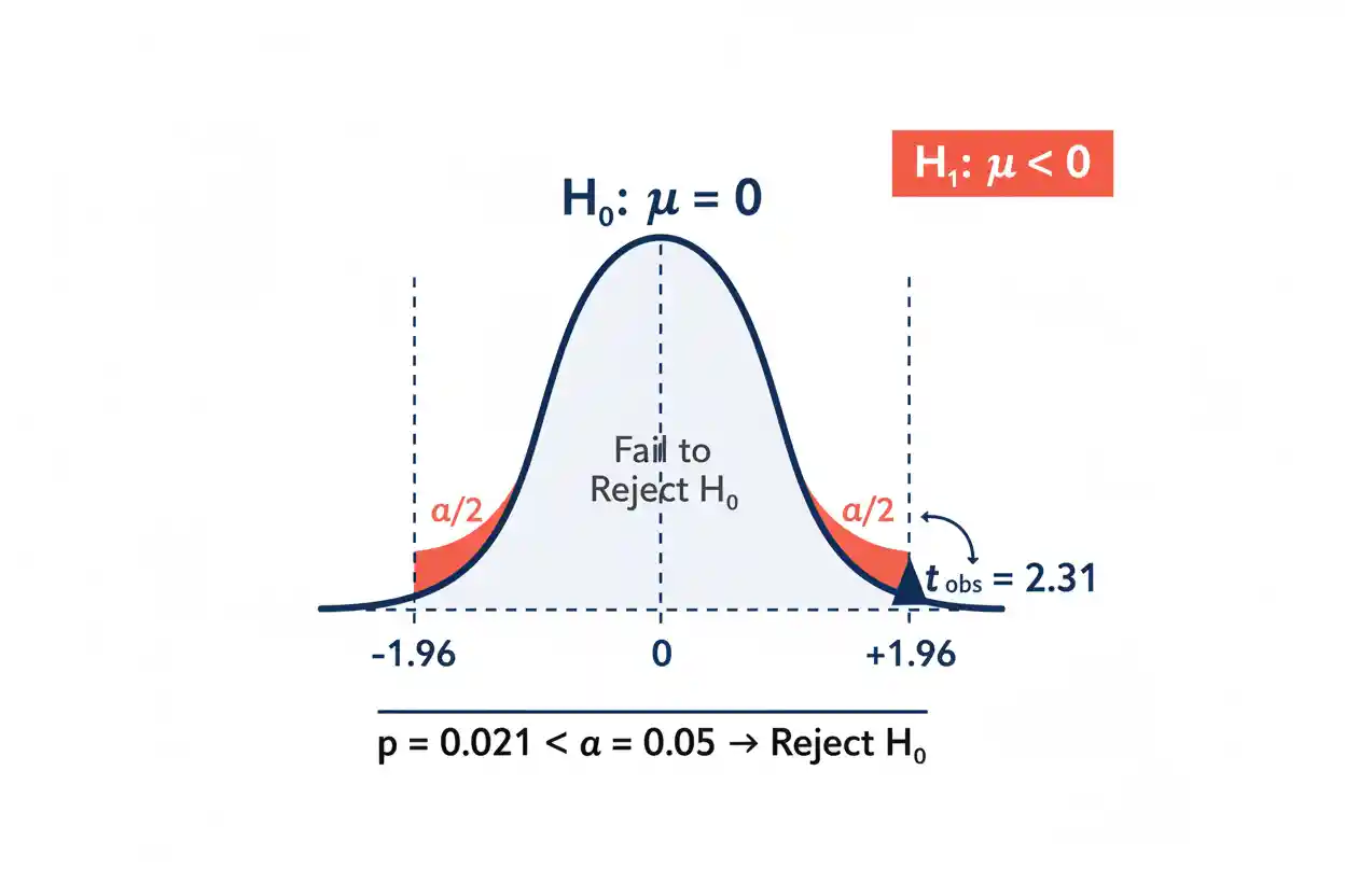

The null hypothesis is a formal statistical statement that specifies the value, relationship, distribution, or model assumption evaluated by a hypothesis test. It is conventionally written as H₀ and usually represents a precise benchmark such as no difference between population means, no association between variables, a population proportion equal to a stated value, or a regression coefficient equal to zero. Statistical testing begins by assuming H₀ is the reference model and asking how unusual the observed sample evidence would be if that model were correct. A test statistic summarizes the discrepancy between the sample result and the null value, while a reference distribution describes how that statistic would behave under H₀.
If the observed result is sufficiently incompatible with the null model according to a prespecified significance level, H₀ is rejected; otherwise, the correct conclusion is to fail to reject H₀. Failing to reject is not the same as proving H₀ true, just as rejecting H₀ does not prove a particular alternative explanation with certainty. The null hypothesis is therefore best understood as the explicit statistical claim against which evidence is evaluated rather than as a statement researchers necessarily believe to be true. Its exact form depends on the parameter and statistical procedure being studied.
The concept is foundational throughout Statistics & Probability and especially within Inference & Regression, where sample evidence is used to evaluate claims about unknown population quantities.
What Is a Null Hypothesis?
A null hypothesis is a mathematical statement about one or more population parameters. It defines the condition assumed when deriving the sampling distribution used by a statistical test.
A simple example concerns a population mean μ. Suppose a manufacturer claims that the mean fill weight of a product is 500 grams. A null hypothesis could be:
H₀: μ = 500
The corresponding alternative might be:
H₁: μ ≠ 500
The test does not begin by assigning probabilities to these two hypotheses. Instead, it temporarily treats H₀ as the reference assumption and asks whether the observed sample statistic would be unusually far from 500 if the population mean really were 500.
The null hypothesis therefore provides the benchmark against which the sample discrepancy is measured.
Why Is It Called the Null Hypothesis?
The word null reflects the historical use of H₀ to represent no effect, no difference, or no association. For example:
H₀: μ₁ − μ₂ = 0
states that two population means do not differ.
Similarly:
H₀: β₁ = 0
can state that a regression predictor has no linear coefficient under a specified model.
However, H₀ does not always have to equal zero. A test could examine:
H₀: μ = 100
or:
H₀: p = 0.40
or:
H₀: μ₁ − μ₂ = 5
The defining feature is not that the null value must literally be zero. It is that H₀ specifies the parameter condition used as the reference for the test.
Null Hypothesis Notation
The null hypothesis is conventionally written:
H₀
The subscript zero distinguishes it from an alternative hypothesis, often written:
H₁
or:
Hₐ
A complete hypothesis test should define both statements before interpreting the data.
For a two-sided population-mean test:
H₀: μ = μ₀
H₁: μ ≠ μ₀
For a right-tailed test:
H₀: μ = μ₀
H₁: μ > μ₀
For a left-tailed test:
H₀: μ = μ₀
H₁: μ < μ₀
The precise formulation determines which sample outcomes count as evidence against H₀.
Null Hypothesis for a Population Mean
Suppose a business process is designed to produce an average completion time of 30 minutes. The population parameter is:
μ = true population mean completion time
A two-sided null hypothesis could be:
H₀: μ = 30
with:
H₁: μ ≠ 30
If the sample mean is:
x̄ = 33
the raw difference from the null value is:
x̄ − μ₀ = 33 − 30 = 3
A statistical test then asks whether a three-minute sample difference is sufficiently large relative to the sampling variability expected under H₀.
The raw difference alone is not enough. A three-minute deviation can be compelling when the sample mean is highly precise and unremarkable when sampling variability is large.
Null Hypothesis and the Test Statistic
A test statistic standardizes or otherwise summarizes the discrepancy between observed data and H₀.
A generic standardized structure is:
Test statistic = (estimate − null value) / standard error
For a sample mean in an appropriate setting:
statistic = (x̄ − μ₀) / SE(x̄)
If:
x̄ = 33
μ₀ = 30
and:
SE(x̄) = 1
then:
statistic = (33 − 30) / 1
statistic = 3
The observed mean lies three standard errors above the null value.
If the standard error were instead 5:
statistic = (33 − 30) / 5
statistic = 0.6
The same three-unit raw discrepancy now represents much weaker evidence against H₀.
Hypothesis testing therefore evaluates effect magnitude relative to sampling uncertainty.
Worked Example: One-Sample Mean Test
Suppose a company claims that average processing time is:
μ₀ = 50 minutes
A random sample produces:
n = 100
x̄ = 52 minutes
Assume for this example that the relevant standard error is:
SE(x̄) = 0.8
The hypotheses are:
H₀: μ = 50
H₁: μ ≠ 50
The standardized statistic is:
z = (52 − 50) / 0.8
z = 2 / 0.8
z = 2.5
A two-sided standard-normal procedure at α = 0.05 uses approximate critical values:
−1.96 and +1.96
Since:
2.5 > 1.96
the observed statistic falls in the rejection region.
The conclusion is to reject H₀ at the 5% significance level. The data provide evidence that the population mean differs from 50.
This does not prove exactly what the true mean is, nor does it imply there is a 5% probability that H₀ is true.
Rejecting the Null Hypothesis
Rejecting H₀ means that the observed data are sufficiently incompatible with the null model according to the chosen test and significance threshold.
Suppose:
H₀: μ = 50
and the test returns:
p = 0.012
with:
α = 0.05
Because:
0.012 < 0.05
the decision is:
Reject H₀
A careful contextual statement might be:
The sample provides statistically significant evidence that the population mean differs from 50.
This is more accurate than saying:
H₀ has been proven false.
Statistical tests make decisions under uncertainty. A rejection procedure is designed to have a controlled probability of rejecting H₀ when it is actually true, subject to the model assumptions.
Failing to Reject the Null Hypothesis
Suppose instead the test produces:
p = 0.28
with:
α = 0.05
Then:
p > α
and the decision is:
Fail to reject H₀
This means the observed sample does not provide sufficiently strong evidence against the null model at the selected significance level.
It does not mean:
H₀ is proven true.
Nor does it mean:
the groups are definitely identical.
A nonsignificant result can arise because H₀ is approximately correct, because the true departure is small, because the sample is too small or noisy, or because the test has limited power for the relevant alternative.
The phrase fail to reject accurately preserves that uncertainty.
Why “Accept H₀” Is Often Misleading
Traditional hypothesis testing is generally constructed to determine whether evidence is strong enough to reject H₀. It does not ordinarily provide a symmetric mechanism for proving the exact null value.
Imagine testing:
H₀: μ = 100
and obtaining:
x̄ = 100.2
with a small sample.
The data may be consistent with μ = 100, but they may also be consistent with nearby values such as 99, 101, or 102 depending on the uncertainty.
A nonsignificant result therefore cannot usually distinguish exact equality from insufficient precision.
When the scientific objective is to demonstrate that effects are sufficiently small, equivalence testing or another procedure explicitly designed for that question is generally more appropriate than treating failure to reject as proof of equality.
The Null Hypothesis and the P-Value
The p-value is calculated conditional on H₀. Conceptually, it asks how unusual the observed test statistic—or a value at least as extreme according to the test definition—would be if the null model were correct.
A simplified two-sided interpretation is:
p-value = P(result at least this extreme | H₀)
It is not:
P(H₀ is true | data)
Those two probabilities reverse the conditioning and have different meanings.
If:
p = 0.03
the correct interpretation is that, under H₀ and the statistical model, outcomes at least as extreme as the observed result would occur with probability 0.03 according to the test definition.
It is incorrect to say:
There is a 3% probability that H₀ is true.
The Null Hypothesis and Significance Level
The significance level α establishes the rejection threshold before the observed test result is interpreted.
Common choices include:
α = 0.10
α = 0.05
α = 0.01
The decision rule using a p-value is:
If p ≤ α, reject H₀.
If p > α, fail to reject H₀.
The significance level also relates to the probability of a Type I error under H₀.
If:
α = 0.05
then a properly calibrated test has a 5% probability of entering the rejection region when H₀ is true, under the assumptions defining that procedure.
Changing α after observing the data simply to obtain a desired conclusion undermines the intended error-control interpretation.
Null Hypothesis and Critical Values
The p-value approach and critical-value approach are equivalent decision frameworks when they use the same statistical test and α.
Suppose a two-sided z test has:
α = 0.05
The approximate critical values are:
−1.96 and +1.96
The rule is:
Reject H₀ if z < −1.96 or z > 1.96
If:
z = 2.30
the statistic crosses the upper critical value and H₀ is rejected.
If:
z = 1.40
the statistic remains inside the non-rejection region.
The critical boundary controls the test decision, while H₀ determines the reference distribution from which that boundary is obtained.
One-Sided Null Hypotheses
Some research questions have a directional alternative.
Suppose a new process is claimed to increase mean output above 100 units.
A right-tailed test might use:
H₀: μ = 100
H₁: μ > 100
Only unusually large sample means count as evidence in the direction specified by H₁.
For a left-tailed problem:
H₀: μ = 100
H₁: μ < 100
only sufficiently low values count against H₀.
A directional alternative should be justified by the research question before examining the sample. Choosing the tail after seeing the direction of the observed result can inflate false-positive risk.
Two-Sided Null Hypotheses
A two-sided alternative is appropriate when deviations in either direction matter.
For example:
H₀: μ = 100
H₁: μ ≠ 100
Evidence can come from a sample mean substantially above or below 100.
At α = 0.05, the rejection probability is typically divided between both tails of a symmetric reference distribution.
For a standard normal test:
0.025 in the lower tail
0.025 in the upper tail
giving approximate critical values:
±1.96
A two-sided test therefore generally requires a more extreme statistic in one direction than a one-sided test using the same total α.
Null Hypothesis in a One-Sample T-Test
A One-Sample T-Test commonly evaluates whether an unknown population mean equals a specified value when the population standard deviation is not known and the standard error is estimated from the sample.
The null hypothesis is typically:
H₀: μ = μ₀
The test statistic is:
t = (x̄ − μ₀) / (s / √n)
where s is the sample standard deviation.
Suppose:
x̄ = 104
μ₀ = 100
s = 12
n = 36
Then:
SE(x̄) = 12 / √36
SE(x̄) = 2
and:
t = (104 − 100) / 2
t = 2
The statistic is then evaluated using the appropriate t distribution with its corresponding degrees of freedom.
Null Hypothesis in a One-Sample Z-Test
A One-Sample Z-Test can also evaluate a population mean against a specified null value when the conditions for the z procedure are satisfied.
A common formulation is:
H₀: μ = μ₀
with statistic:
z = (x̄ − μ₀) / (σ / √n)
where σ is the relevant population standard deviation in the classical known-σ formulation.
The logic is the same: H₀ supplies the population value used to center the reference distribution, while the standardized statistic measures how far the observed sample mean lies from that benchmark.
The choice between t and z procedures depends on their respective assumptions rather than on whether the researcher prefers one reference distribution.
Null Hypothesis for a Population Proportion
Suppose a business believes that 40% of customers choose a particular option.
The parameter is:
p = true population proportion
The null hypothesis can be:
H₀: p = 0.40
A two-sided alternative is:
H₁: p ≠ 0.40
If a sample produces:
p̂ = 0.46
the observed difference is:
p̂ − p₀ = 0.46 − 0.40
p̂ − p₀ = 0.06
The statistical test then evaluates whether this six-percentage-point sample departure is large relative to the sampling variability predicted under:
p = 0.40
Again, the null value determines the reference calculation.
Null Hypothesis for Two Means
Suppose the research question asks whether two population means differ.
A conventional null can be written:
H₀: μ₁ = μ₂
Equivalently:
H₀: μ₁ − μ₂ = 0
The alternative may be:
H₁: μ₁ − μ₂ ≠ 0
The second form makes the null effect explicit: the population mean difference is zero.
However, zero need not be the only possible benchmark. If the question concerns whether one mean exceeds another by exactly five units, the null could instead be:
H₀: μ₁ − μ₂ = 5
The null statement should reflect the actual inferential claim being evaluated.
Null Hypothesis in Multiple Regression
In Multiple Regression, a common null hypothesis for an individual predictor is:
H₀: βⱼ = 0
This states that predictor xⱼ has zero conditional linear coefficient in the specified population regression model.
The alternative may be:
H₁: βⱼ ≠ 0
A common test statistic is:
t = bⱼ / SE(bⱼ)
when the null value is zero.
Rejecting H₀ provides evidence that the population coefficient differs from zero under the regression model and its assumptions.
It does not prove that xⱼ causes Y. Regression coefficients can reflect confounding, model specification, measurement structure, or other noncausal relationships.
Overall Null Hypothesis in Regression
A multiple regression model can also be tested as a group.
With k predictors, an overall null may be:
H₀: β₁ = β₂ = … = βₖ = 0
The alternative is that at least one population slope coefficient is nonzero.
This asks whether the complete set of predictors provides evidence of linear predictive information beyond an intercept-only model.
Rejecting this overall null does not imply that every coefficient differs from zero. It establishes evidence against the joint restriction that all slopes are zero.
Individual coefficients require their own inference if separate conclusions are desired.
Null Hypothesis in Logistic Regression
In Logistic Regression, an individual predictor coefficient can also be tested using:
H₀: βⱼ = 0
Because logistic coefficients operate on the log-odds scale, the corresponding null odds ratio is:
OR = e⁰
OR = 1
Thus:
H₀: βⱼ = 0
is equivalent to:
H₀: ORⱼ = 1
for the specified predictor comparison.
Rejecting H₀ provides evidence that the predictor is conditionally associated with the outcome according to the fitted logistic model.
It does not mean that the odds ratio is necessarily large or practically important.
Null Hypothesis and Effect Size
The null hypothesis usually identifies a reference value, while Effect Size quantifies the magnitude of the observed or estimated phenomenon.
Suppose a standardized mean difference is:
d = 0.08
In a very large sample, this small effect could be statistically distinguishable from a null value of zero.
Alternatively, a study might estimate:
d = 0.80
but have a small sample and wide uncertainty, resulting in insufficient evidence to reject H₀.
Therefore:
statistical significance ≠ effect magnitude
The null hypothesis asks whether the evidence is compatible with a specified benchmark. Effect size asks how large the estimated difference or relationship is.
Both pieces of information can be important.
Statistical Significance vs Practical Importance
Suppose a large dataset estimates a mean difference of:
0.2 units
with an extremely small standard error.
A test might strongly reject:
H₀: difference = 0
Even so, a difference of 0.2 units may have no practical consequence.
Conversely, a small pilot study might estimate a difference of 15 units but fail to reject H₀ because uncertainty is very large.
A hypothesis-test decision therefore should never be used as a substitute for assessing practical magnitude.
Decision-making should consider the effect estimate, confidence interval, costs, benefits, and real-world threshold of importance.
Type I Error
A Type I error occurs when a test rejects H₀ even though H₀ is actually true.
Symbolically:
Type I error = reject H₀ when H₀ is true
The probability of this error under a correctly calibrated procedure is controlled by α:
P(Type I error | H₀ true) = α
If:
α = 0.05
then the testing procedure is designed so that, when H₀ is true and assumptions hold, approximately 5% of repeated tests would reject it.
This does not mean that every observed rejection has a 5% probability of being wrong.
The probability refers to repeated-sampling behavior under H₀.
Type II Error
A Type II error occurs when a test fails to reject H₀ even though a particular alternative is true.
Conceptually:
Type II error = fail to reject H₀ when H₀ is false
Its probability is commonly denoted:
β
Statistical power is:
Power = 1 − β
Power depends on factors including:
- true effect magnitude
- sample size
- variability
- significance threshold
- statistical design
A nonsignificant result from a low-powered study may therefore provide little evidence that the null condition is approximately true.
The Null Hypothesis Is Not Necessarily the Researcher’s Belief
Researchers do not have to believe H₀ for it to serve as the reference model.
Suppose a scientist strongly expects that a treatment changes an outcome. The formal test may still begin with:
H₀: treatment effect = 0
The role of H₀ is procedural: it specifies the distribution used to judge how surprising the observed evidence would be in the absence of the hypothesized effect.
This is why calling H₀ the “default belief” can sometimes be misleading.
It is better described as the benchmark or reference claim used by the testing procedure.
The Null Hypothesis Must Be Specific Enough to Test
A useful null hypothesis must define the conditions needed to derive the relevant test statistic’s reference distribution.
A vague statement such as:
H₀: nothing unusual is happening
is not statistically sufficient.
A precise statement might be:
H₀: μ = 25
or:
H₀: p = 0.60
or:
H₀: β₁ = 0
or:
H₀: μ₁ − μ₂ = 0
The hypothesis should specify the parameter and null value clearly enough that the corresponding probability model can be constructed.
Composite Null Hypotheses
Not every null hypothesis consists of exactly one parameter value.
Some procedures evaluate composite hypotheses containing a set of parameter values.
For example, a one-sided formulation might conceptually involve:
H₀: μ ≤ μ₀
against:
H₁: μ > μ₀
The boundary value μ = μ₀ commonly determines the reference distribution used to calibrate the test.
Other statistical models can involve even more complex restrictions across multiple parameters.
The simple equality null is therefore an important foundation, but hypothesis testing is not limited to one-point null statements.
Choosing H₀ Before Examining the Result
The hypothesis and testing direction should ideally be established from the scientific or decision question before examining whether the sample result is favorable.
Suppose the original research question is whether a treatment differs from control in either direction. The natural hypotheses are:
H₀: difference = 0
H₁: difference ≠ 0
If the sample later happens to show a positive difference, changing the alternative to:
H₁: difference > 0
solely to obtain a smaller p-value alters the procedure after seeing the evidence.
Such data-dependent choices can increase false-positive rates and weaken the intended interpretation of α.
Sample Size and the Null Hypothesis
The null hypothesis itself does not become more or less true because sample size changes. What changes is the amount of information available to distinguish the null value from nearby alternatives.
Suppose the true population difference is only:
0.10
A small study may be unable to distinguish that value from zero.
A huge study may estimate the difference extremely precisely and strongly reject:
H₀: difference = 0
even though the effect remains numerically tiny.
This is another reason that rejecting H₀ should not automatically be described as discovering an important effect.
Confidence Intervals and H₀
Confidence intervals can often be connected directly to a corresponding two-sided hypothesis test.
Suppose the parameter is a mean difference and the null is:
H₀: Δ = 0
If a compatible 95% confidence interval is:
2.0 to 6.0
then zero is excluded, which generally corresponds to rejection at:
α = 0.05
for the matching two-sided procedure.
If the interval is:
−1.5 to 4.0
zero is included, corresponding to failure to reject the zero-difference null with the compatible test.
The interval provides more information than the binary decision because it shows which parameter magnitudes remain reasonably compatible with the data under the interval procedure.
Null Values Depend on the Statistic
Zero is a common null value, but not every effect measure uses zero.
For a mean difference:
H₀ value = 0
For a regression coefficient:
H₀ value = 0
For a correlation:
H₀ value often = 0
For a risk ratio:
H₀ value = 1
For an odds ratio:
H₀ value = 1
For a proportion:
H₀ can be any specified valid probability such as 0.50
The relevant null value follows from what constitutes no difference or the benchmark of interest on the scale of the parameter.
A Significant Result Does Not Prove H₁
Suppose:
H₀: μ = 100
and a test rejects H₀.
Many alternative values could explain the evidence:
μ = 101
μ = 105
μ = 120
The test against H₀ alone does not prove which particular alternative is correct.
Similarly, a significant association can result from multiple possible mechanisms.
Estimation, confidence intervals, model diagnostics, replication, and substantive reasoning are needed to understand what the departure from H₀ actually looks like.
Hypothesis testing is evidence against a benchmark, not a complete explanation of the data-generating process.
Failure to Reject Does Not Show Equivalence
Suppose two treatments differ by an estimated:
1 unit
but the confidence interval ranges from:
−8 to +10
A conventional test may fail to reject:
H₀: difference = 0
Yet the data remain compatible with differences that could be practically substantial in either direction.
It would therefore be incorrect to conclude that the treatments are equivalent.
To demonstrate practical equivalence, researchers generally need to define a range of differences considered negligible and use an inferential procedure designed to test whether the effect lies within that range.
Common Misconceptions
A common misconception is that the null hypothesis is the probability that nothing is happening. H₀ is a mathematical statement about parameters or a model, not a probability.
Another mistake is interpreting a p-value as:
P(H₀ is true)
A frequentist p-value is instead calculated under H₀.
A third misconception is that failing to reject H₀ proves it true. A nonsignificant result may simply reflect insufficient information.
Researchers also sometimes believe rejecting H₀ proves the exact alternative they hoped for. Rejection only establishes evidence against the specified null under the testing procedure.
Another error is equating statistical significance with practical importance. Tiny effects can reject H₀ in very large samples.
Finally, the null hypothesis should not be changed after seeing the result merely to obtain a preferred test outcome.
How to Write a Null Hypothesis
First identify the population parameter of interest. Examples include:
μ
p
μ₁ − μ₂
β₁
Then define the benchmark value or relationship being evaluated.
For a population mean:
H₀: μ = 50
For a population proportion:
H₀: p = 0.30
For two means:
H₀: μ₁ − μ₂ = 0
For a regression coefficient:
H₀: β₁ = 0
Next specify the alternative according to the research question.
Two-sided:
H₁: parameter ≠ null value
Right-sided:
H₁: parameter > null value
Left-sided:
H₁: parameter < null value
The hypothesis should be chosen before interpreting the observed sample evidence.
Practical Example: Quality Control
Suppose bottles are designed to contain an average of 1,000 milliliters.
The hypotheses are:
H₀: μ = 1,000
H₁: μ ≠ 1,000
A sample gives:
x̄ = 998.5
Whether this difference is statistically meaningful depends on the standard error.
If:
SE(x̄) = 0.5
then:
z = (998.5 − 1,000) / 0.5
z = −3
The sample mean is three standard errors below the null value.
If:
SE(x̄) = 5
then:
z = −1.5 / 5
z = −0.3
The same raw difference now provides very little evidence against H₀.
This illustrates why hypothesis tests combine discrepancy with precision.
Practical Example: Conversion Rate
Suppose a website historically has a conversion probability of:
p₀ = 0.08
A new version is tested with:
H₀: p = 0.08
H₁: p > 0.08
If the sample conversion rate is:
p̂ = 0.085
the raw increase is only:
0.005
or 0.5 percentage points.
Whether H₀ is rejected depends on sample size and sampling variability.
With a small sample, the evidence may be weak. With millions of observations, the same 0.5-point difference could be estimated very precisely.
Even if statistically significant, the business should still evaluate whether the improvement is economically meaningful.
Practical Example: Regression Coefficient
Suppose a model estimates:
b₁ = 2.4
with:
SE(b₁) = 0.8
The null hypothesis is:
H₀: β₁ = 0
The test statistic is:
t = 2.4 / 0.8
t = 3
A statistic of this magnitude may provide substantial evidence against H₀ depending on the appropriate reference distribution and degrees of freedom.
The result supports a nonzero conditional relationship between the predictor and response under the model.
It does not by itself establish that changing the predictor by one unit would causally change the response by 2.4 units.
Frequently Asked Questions
What is a null hypothesis?
A null hypothesis is a formal statistical statement used as the reference condition in a hypothesis test. It is conventionally written H₀.
What is an example of a null hypothesis?
For a population mean:
H₀: μ = 100
This states that the population mean equals 100.
Does the null hypothesis always mean no difference?
No. Zero difference is common, but H₀ can specify any relevant benchmark, such as:
H₀: μ = 50
or:
H₀: p = 0.30
What is the difference between H₀ and H₁?
H₀ is the reference hypothesis being tested. H₁ represents the alternative condition supported when the data provide sufficiently strong evidence against H₀.
What does rejecting H₀ mean?
It means the observed sample evidence is sufficiently incompatible with the null model according to the specified test and significance level.
Does rejecting H₀ prove H₁?
No. It provides evidence against H₀ but does not prove one exact alternative explanation with certainty.
What does failing to reject H₀ mean?
It means the data do not provide sufficiently strong evidence against H₀ at the chosen threshold.
Does failing to reject H₀ prove it is true?
No. Lack of significance can reflect limited sample size, large variability, a small true effect, or a null model that is approximately correct.
Is a p-value the probability that H₀ is true?
No. A p-value is calculated assuming H₀ and describes the probability of obtaining a result at least as extreme as the observed result according to the test definition.
Why is zero often used in H₀?
For differences and many regression coefficients, zero represents no difference or no linear effect on the parameter’s scale.
Can a null value equal 1?
Yes. Ratios such as odds ratios and risk ratios commonly use 1 as the no-association null value.
What is H₀ in regression?
For an individual regression coefficient, a common null is:
H₀: βⱼ = 0
What is H₀ in logistic regression?
A common coefficient null is:
H₀: βⱼ = 0
which corresponds to:
OR = 1
for the associated odds ratio.
What is a Type I error?
A Type I error occurs when H₀ is rejected even though it is actually true under the model.
What is a Type II error?
A Type II error occurs when the test fails to reject H₀ even though the relevant alternative is true.
Can a tiny effect reject H₀?
Yes. With a sufficiently large and precise sample, even a very small departure from the null value can be statistically detectable.
Should H₀ be chosen after seeing the data?
The core hypothesis and testing direction should generally be established from the research question before interpreting the observed result.
Is statistical significance the same as practical significance?
No. Rejecting H₀ concerns evidence against a statistical benchmark. Practical significance concerns whether the estimated effect is large enough to matter.
Key Takeaway
The null hypothesis is the formal reference statement evaluated by a statistical test. It is written:
H₀
and commonly takes forms such as:
H₀: μ = μ₀
H₀: p = p₀
H₀: μ₁ − μ₂ = 0
H₀: βⱼ = 0
Sample evidence is summarized with a test statistic and compared with the distribution expected under H₀. If the result is sufficiently extreme according to a prespecified significance threshold, H₀ is rejected. Otherwise, the appropriate conclusion is to fail to reject H₀.
Neither decision establishes certainty. Rejecting H₀ does not assign a probability to the hypothesis or prove a particular causal explanation, while failing to reject H₀ does not demonstrate that the null condition is exactly true. The null hypothesis is most useful when treated as a precise statistical benchmark that organizes evidence, uncertainty, error rates, and inferential decisions while remaining separate from effect magnitude and practical importance.



