Logistic Regression: Definition, Formula & Example

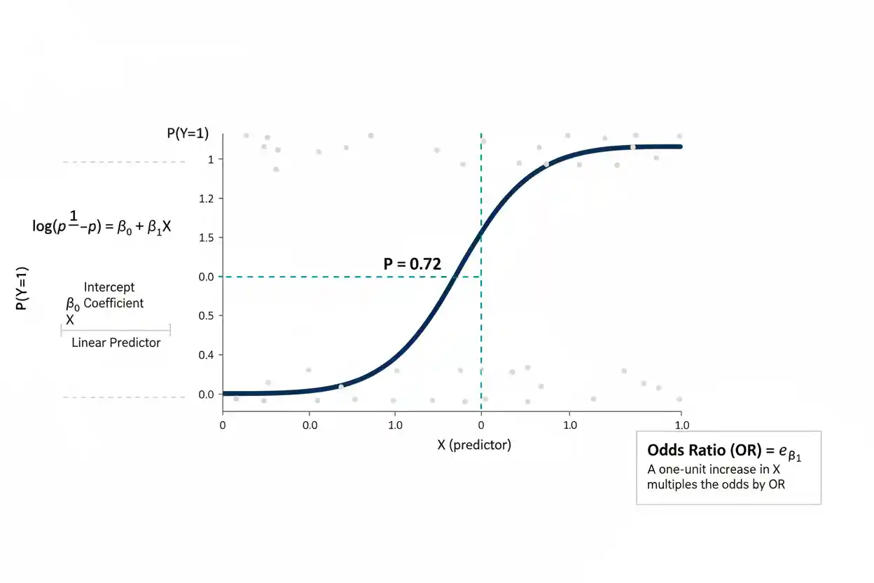
Logistic regression is a statistical model used when an outcome represents membership in one of two categories, commonly coded as 0 and 1. Instead of fitting an unrestricted straight line directly to the binary outcome, the model relates predictors to the log-odds of the event and then converts those log-odds into a probability between 0 and 1. This structure makes logistic regression suitable for questions such as whether a customer converts, a machine fails, an applicant is approved, a patient experiences an event, or a transaction belongs to a specified class. Its coefficients are linear on the log-odds scale, while exponentiating a coefficient converts it into an odds ratio that is often easier to interpret.

Logistic regression can contain continuous predictors, categorical predictors, interactions, and multiple explanatory variables, but the interpretation of each coefficient is conditional on the other variables included in the model. Unlike ordinary linear regression, it is generally estimated by maximum likelihood rather than by minimizing the ordinary sum of squared residuals. It does not require predictors themselves to be normally distributed, but it does rely on assumptions about the sampling structure, model specification, and relationship between continuous predictors and the logit. A fitted probability is also not automatically a classification: converting probabilities into labels requires a separate decision threshold chosen for the application.

Logistic regression belongs to Statistics & Probability and is a central method within Inference & Regression. Its primary role is to model a binary outcome through probabilities, odds, and log-odds while allowing the influence of one or more predictors to be estimated.

What Is Logistic Regression?

Binary logistic regression models the probability that an outcome Y equals 1 rather than 0. If:

Y ∈ {0, 1}

then the model focuses on:

p = P(Y = 1 | X)

The probability of the other outcome is:

P(Y = 0 | X) = 1 − p

A direct linear model such as:

p = β₀ + β₁x

creates an immediate problem because a straight line can generate predictions below 0 or above 1. Probabilities, however, must satisfy:

0 ≤ p ≤ 1

Logistic regression solves this problem by modeling a transformed version of p. The transformation is the logit, or log-odds:

logit(p) = ln[p / (1 − p)]

For one predictor:

ln[p / (1 − p)] = β₀ + β₁x

For several predictors:

ln[p / (1 − p)] = β₀ + β₁x₁ + β₂x₂ + … + βₖxₖ

The right-hand side can take any real value, while the inverse logistic transformation maps that value back into the valid probability range from 0 to 1.

The Logistic Regression Formula

Let the linear predictor be:

η = β₀ + β₁x₁ + β₂x₂ + … + βₖxₖ

The corresponding probability is:

p = 1 / (1 + e^(−η))

Substituting the linear predictor gives:

p = 1 / [1 + e^(−(β₀ + β₁x₁ + β₂x₂ + … + βₖxₖ))]

This function is called the logistic function. Its familiar S shape approaches 0 for very negative values of η and approaches 1 for very positive values, but it never produces a probability below 0 or above 1.

At:

η = 0

the probability is:

p = 1 / (1 + e⁰)

p = 1/2

p = 0.50

Positive values of η correspond to probabilities above 0.50, while negative values correspond to probabilities below 0.50.

This does not mean that 0.50 must be used as a classification threshold. The logistic model produces probabilities; the decision threshold is a separate choice.

Probability, Odds, and Log-Odds

Understanding logistic regression becomes much easier when probability, odds, and log-odds are distinguished.

If an event has probability p, its odds are:

Odds = p / (1 − p)

Suppose:

p = 0.75

Then:

Odds = 0.75 / 0.25

Odds = 3

The event therefore has odds of 3 to 1.

If:

p = 0.20

then:

Odds = 0.20 / 0.80

Odds = 0.25

This can be described as odds of 1 to 4.

Logistic regression takes the natural logarithm of the odds:

Log-odds = ln[p / (1 − p)]

The log-odds can range from:

−∞ to +∞

which makes them suitable for modeling as a linear combination of predictors.

Converting Odds Back to Probability

If the odds are known, probability can be recovered using:

p = Odds / (1 + Odds)

Suppose the odds equal 4:

p = 4 / (1 + 4)

p = 4/5

p = 0.80

If the log-odds equal η, first exponentiate:

Odds = e^η

Then convert to probability:

p = e^η / (1 + e^η)

This is algebraically equivalent to:

p = 1 / (1 + e^(−η))

Both forms represent the same logistic function.

Worked Example With One Predictor

Suppose a fitted logistic regression predicting whether an event occurs has:

β₀ = −2

β₁ = 0.08

The model is:

ln[p / (1 − p)] = −2 + 0.08x

Suppose:

x = 30

The linear predictor is:

η = −2 + 0.08(30)

η = −2 + 2.4

η = 0.4

Convert this to a probability:

p = 1 / (1 + e^(−0.4))

Since:

e^(−0.4) ≈ 0.6703

then:

p ≈ 1 / 1.6703

p ≈ 0.5987

The model therefore predicts an event probability of approximately:

59.9%

for x = 30.

This is a probability prediction, not proof that the event will occur for that particular observation.

Interpreting the Intercept

In a one-predictor model:

ln[p / (1 − p)] = β₀ + β₁x

the intercept β₀ is the predicted log-odds when:

x = 0

Suppose:

β₀ = −2

Then at x = 0:

Log-odds = −2

The corresponding odds are:

Odds = e^(−2)

Odds ≈ 0.1353

and the probability is:

p = 1 / (1 + e²)

p ≈ 0.1192

Thus the predicted event probability at x = 0 is approximately 11.9%.

Whether the intercept has substantive meaning depends on whether x = 0 is a realistic and meaningful predictor value. If zero lies far outside the observed range, the intercept can remain mathematically necessary while having little direct practical interpretation.

Interpreting a Logistic Regression Coefficient

A coefficient β₁ represents the change in log-odds associated with a one-unit increase in x₁, holding the other included predictors constant.

If:

β₁ = 0.08

then a one-unit increase in x changes the log-odds by:

+0.08

This is mathematically precise, but log-odds are often difficult to interpret intuitively. Exponentiating the coefficient produces an odds ratio:

OR = e^β¹

More generally:

OR = e^(β₁)

For:

β₁ = 0.08

the odds ratio is:

OR = e^0.08

OR ≈ 1.083

A one-unit increase in x is therefore associated with multiplying the odds of the event by approximately 1.083, holding the other predictors constant.

This corresponds to about an 8.3% increase in the odds:

(1.083 − 1) × 100% ≈ 8.3%

It does not mean that the probability increases by 8.3 percentage points.

Odds Ratio Interpretation

The exponentiated coefficient is one of the most commonly reported quantities from logistic regression:

OR = e^β

Its interpretation depends on whether it is above, below, or equal to 1.

If:

OR = 1

the predictor produces no change in the modeled odds for a one-unit increase, conditional on the other included predictors.

If:

OR > 1

the odds increase.

If:

OR < 1

the odds decrease.

For example:

OR = 1.50

means the odds are multiplied by 1.50, corresponding to a 50% increase in odds.

If:

OR = 0.70

the odds are multiplied by 0.70, corresponding to a 30% decrease in odds:

(1 − 0.70) × 100% = 30%

Again, odds and probability are not the same quantity.

Why an Odds Ratio Is Not a Probability Ratio

Suppose the baseline probability is:

p₀ = 0.10

The baseline odds are:

0.10 / 0.90 ≈ 0.111

If an exposure doubles the odds:

OR = 2

the new odds are:

0.222

The corresponding probability becomes:

p₁ = 0.222 / 1.222

p₁ ≈ 0.182

The probability rose from 10% to approximately 18.2%, not to 20%.

Now suppose the baseline probability is 0.50. The baseline odds are 1. Doubling the odds gives odds of 2, corresponding to:

p = 2/3

p ≈ 0.667

The probability rises from 50% to about 66.7%.

The same odds ratio can therefore correspond to different probability changes depending on the starting probability.

Interpreting Larger Changes in a Predictor

A coefficient describes a one-unit increase, but the odds ratio for a larger change can be calculated directly.

If:

β₁ = 0.08

then the odds ratio for a 10-unit increase is:

OR₁₀ = e^(10 × 0.08)

OR₁₀ = e^0.8

OR₁₀ ≈ 2.226

Thus a 10-unit increase in x multiplies the odds by approximately 2.23, assuming the modeled logit relationship remains appropriate across that change and the other predictors remain fixed.

This can sometimes be more interpretable than discussing one-unit changes when one unit is substantively tiny.

Logistic Regression With Multiple Predictors

A multiple-predictor logistic model has the form:

ln[p / (1 − p)] = β₀ + β₁x₁ + β₂x₂ + … + βₖxₖ

Each coefficient describes a conditional association.

Suppose:

ln[p / (1 − p)] = −3 + 0.06x₁ + 0.80x₂

where x₁ is continuous and x₂ is coded 0 or 1.

For x₁:

OR = e^0.06 ≈ 1.062

A one-unit increase in x₁ multiplies the odds by approximately 1.062, holding x₂ constant.

For x₂:

OR = e^0.80 ≈ 2.226

Moving from x₂ = 0 to x₂ = 1 multiplies the modeled odds by approximately 2.23, holding x₁ constant.

This conditional interpretation is a fundamental feature of regression modeling.

The broader structure of models containing several explanatory variables is developed separately in Multiple Regression; here the focus remains on the binary-outcome logistic model.

Worked Multiple-Predictor Probability Example

Using:

η = −3 + 0.06x₁ + 0.80x₂

suppose:

x₁ = 40

x₂ = 1

Then:

η = −3 + 0.06(40) + 0.80(1)

η = −3 + 2.4 + 0.8

η = 0.2

Convert this to probability:

p = 1 / (1 + e^(−0.2))

p ≈ 0.5498

The fitted probability is therefore approximately:

55.0%

Now hold x₁ = 40 but change x₂ to 0:

η = −3 + 2.4

η = −0.6

Then:

p = 1 / (1 + e^0.6)

p ≈ 0.3543

The fitted probabilities differ substantially, but the coefficient for x₂ should still be understood primarily as a conditional log-odds difference or odds ratio. Probability differences depend on the values of all predictors because the logistic transformation is nonlinear.

Categorical Predictors

Categorical predictors can be included by representing categories with indicator variables.

Suppose a predictor has three categories:

• A
• B
• C

If A is chosen as the reference category, define indicators for B and C.

The model can be written:

logit(p) = β₀ + βBIB + βCIC

where IB equals 1 for category B and 0 otherwise, while IC equals 1 for category C and 0 otherwise.

Then:

e^(βB)

is the odds ratio comparing B with reference category A, holding other predictors constant.

Similarly:

e^(βC)

compares C with A.

Changing the reference category changes the numerical coefficient representation but does not change the fitted probabilities produced by the same underlying model.

Logistic Regression and Binary Outcomes

The ordinary binary logistic model assumes the response has two possible states. Common codings are:

0 = event absent

1 = event present

The coding determines which event probability is modeled.

If the coding is reversed, the signs of the relevant coefficients and the interpretation of the odds ratios also reverse.

For example, a model predicting:

P(Y = 1)

may describe the probability of approval.

Reversing the coding could instead model:

P(Y = 1) = probability of rejection

The statistical information is closely related, but the interpretation changes substantially. The event category should therefore always be defined explicitly.

How Logistic Regression Is Estimated

Ordinary linear regression commonly estimates coefficients by minimizing squared residuals. Binary logistic regression is generally estimated using maximum likelihood.

For observation i with outcome:

yᵢ ∈ {0,1}

and modeled event probability pᵢ, the likelihood contribution is:

pᵢ^(yᵢ) × (1 − pᵢ)^(1 − yᵢ)

Across n independent observations:

L(β) = Π [pᵢ^(yᵢ) × (1 − pᵢ)^(1 − yᵢ)]

The coefficient estimates are chosen to maximize this likelihood.

It is usually computationally convenient to maximize the log-likelihood:

ln L(β) = Σ[yᵢ ln(pᵢ) + (1 − yᵢ)ln(1 − pᵢ)]

There is generally no simple closed-form formula that directly produces all logistic regression coefficients. Numerical optimization methods are therefore used.

Maximum Likelihood Intuition

Maximum likelihood asks which coefficient values make the observed binary outcomes most plausible under the model.

If an observation has:

y = 1

a fitted probability near 1 contributes more favorably to the likelihood than a fitted probability near 0.

If:

y = 0

a fitted probability near 0 contributes more favorably.

The fitting process searches for coefficients that collectively assign high probability to the outcomes actually observed while respecting the logistic functional form.

This is different from simply choosing a line that minimizes squared vertical distances from 0 and 1.

Logistic Regression vs Linear Regression

Both logistic and linear regression use predictors to model an outcome, but their outcome structures and interpretations differ.

A standard linear regression takes the form:

E(Y | X) = β₀ + β₁x₁ + … + βₖxₖ

and is naturally suited to quantitative outcomes when its assumptions are appropriate.

Binary logistic regression models:

logit[P(Y = 1 | X)] = β₀ + β₁x₁ + … + βₖxₖ

The logistic transformation keeps fitted probabilities between 0 and 1 and recognizes that the variance of a binary outcome depends on its probability.

Using ordinary linear regression for a binary response can produce impossible predicted probabilities and inappropriate error assumptions. Logistic regression addresses these structural problems directly.

Logistic Regression Does Not Require Normal Predictors

A widespread misconception is that predictor variables must be normally distributed for logistic regression.

They do not.

Predictors can be skewed, binary, categorical, or otherwise non-normal. The model does not assume:

X ∼ Normal

for every predictor.

Likewise, logistic regression does not assume normally distributed residuals in the same way as ordinary Gaussian linear regression.

Its assumptions concern the response distribution conditional on predictors, the functional form of the model, the dependence structure, and other characteristics relevant to likelihood-based inference.

Linearity in the Logit

Logistic regression does not assume probability is a linear function of a continuous predictor.

Instead, the basic model assumes the log-odds are linear in the predictor unless nonlinear terms are explicitly included:

logit(p) = β₀ + β₁x

This means a one-unit increase in x corresponds to a constant additive change β₁ in log-odds and a constant multiplicative change e^β¹ in odds.

The probability change itself is not constant.

For example, increasing x by one unit might change the fitted probability from 0.10 to 0.11 at one point and from 0.48 to 0.50 at another. The same coefficient can generate different probability differences because the logistic curve is nonlinear.

If the logit relationship is strongly nonlinear, transformations, splines, polynomial terms, or another suitable modeling approach may be needed.

Independence of Observations

The simplest logistic regression assumes observations contribute appropriately independent information conditional on the model.

Repeated measurements from the same person, students clustered within schools, customers nested within regions, or observations collected sequentially over time can violate this assumption if their dependence is ignored.

A dataset containing 10,000 rows does not necessarily contain the information equivalent of 10,000 independent observations.

When clustering or repeated measurements are present, specialized methods such as mixed-effects logistic models, generalized estimating equations, cluster-robust inference, or other appropriate approaches may be necessary.

The correct method depends on how the dependence arises.

Multicollinearity

When predictors are strongly related to one another, individual logistic regression coefficients can become difficult to estimate precisely.

Suppose x₁ and x₂ contain almost the same information. The model may predict probabilities reasonably well but struggle to determine how much of the relationship should be attributed to β₁ versus β₂.

Consequences can include:

• large standard errors
• unstable coefficient estimates
• sign changes across specifications
• wide confidence intervals

Multicollinearity does not mean the logistic function itself has failed. It means the data contain limited independent information for separating the effects of highly redundant predictors.

Interpretation of individual coefficients therefore requires attention to predictor relationships.

Complete and Quasi-Complete Separation

A distinctive issue in logistic regression occurs when a predictor or combination of predictors perfectly separates the two outcome classes.

Suppose every observation with:

x > 10

has Y = 1, while every observation with:

x ≤ 10

has Y = 0.

The data can then be perfectly separated. Under ordinary maximum likelihood estimation, coefficient estimates may diverge toward extremely large magnitudes rather than settling at finite values.

Quasi-complete separation describes a closely related situation in which separation is nearly perfect.

Warnings about very large coefficients, enormous standard errors, or failure of an optimization algorithm to converge should not simply be ignored. Penalized or specialized estimation methods may be required.

Sample Size and Sparse Outcomes

Logistic regression requires enough information to estimate the specified parameters reliably. The total sample size matters, but so does the number of observations in each outcome category.

A dataset with 100,000 observations can still provide little information about a rare event if only a handful of cases have:

Y = 1

Similarly, a model containing many predictors relative to the available events can produce unstable estimates and overfitting.

There is no universal sample-size threshold that guarantees valid logistic regression. Adequacy depends on event frequency, number and complexity of predictors, effect sizes, collinearity, model structure, and the intended use of the estimates or predictions.

Hypothesis Testing in Logistic Regression

Individual coefficients are often tested against a Null Hypothesis such as:

H₀: βⱼ = 0

Against a two-sided alternative:

H₁: βⱼ ≠ 0

Under H₀:

e^(βⱼ) = 1

so the corresponding conditional odds ratio equals 1.

Several inferential approaches can be used, including Wald tests, likelihood-ratio tests, and score tests. They are related but not identical and can behave differently, particularly in small or irregular samples.

A hypothesis test addresses evidence about a coefficient. It does not determine whether the associated effect is practically important.

Wald Test and Critical Values

A common large-sample Wald statistic takes the approximate form:

z = β̂ⱼ / SE(β̂ⱼ)

when testing:

H₀: βⱼ = 0

The observed standardized statistic can be compared with an appropriate Critical Value.

For a two-sided large-sample procedure at:

α = 0.05

the familiar standard-normal cutoffs are approximately:

−1.96 and +1.96

If:

|z| > 1.96

the coefficient crosses the conventional rejection boundary for that test.

This does not mean the coefficient itself must exceed 1.96. The statistic divides the estimate by its standard error, so magnitude and precision both affect the inferential result.

Confidence Intervals for Logistic Coefficients

A large-sample confidence interval for a coefficient can be approximated by:

β̂ⱼ ± z* × SE(β̂ⱼ)

For a normal-based 95% interval:

z* ≈ 1.96

Suppose:

β̂ = 0.50

SE(β̂) = 0.20

Then:

Lower ≈ 0.50 − 1.96(0.20)

Lower ≈ 0.108

and:

Upper ≈ 0.50 + 1.96(0.20)

Upper ≈ 0.892

The approximate coefficient interval is:

0.108 to 0.892

Exponentiating both endpoints gives an odds-ratio interval:

e^0.108 ≈ 1.11

e^0.892 ≈ 2.44

so the approximate OR interval is:

1.11 to 2.44

Because 1 is excluded from the odds-ratio interval, this aligns with rejecting β = 0 in the corresponding compatible two-sided large-sample test.

Odds Ratio Confidence Intervals

Because odds ratios are obtained from:

OR = e^β

a confidence interval for β can be transformed by exponentiating its endpoints.

If:

β interval = [L, U]

then:

OR interval = [e^L, e^U]

Suppose:

β̂ = −0.40

with a coefficient interval:

−0.70 to −0.10

Then:

OR = e^(−0.40) ≈ 0.67

and the interval becomes approximately:

e^(−0.70) to e^(−0.10)

0.50 to 0.90

The odds are estimated to be lower as the predictor increases, conditional on the other variables in the model.

The interval also communicates uncertainty that the point estimate alone cannot show.

Statistical Significance vs Effect Size

A logistic coefficient can be statistically significant while representing a small effect, especially in a large sample. Conversely, a large estimated odds ratio can remain highly uncertain when the relevant outcome is rare or the sample is small.

The broader concept of Effect Size therefore remains separate from statistical significance.

For example:

OR = 1.03

might be estimated extremely precisely in a massive dataset and produce a tiny p-value.

Another study might estimate:

OR = 2.5

with a very wide confidence interval because only a few events occurred.

The first has stronger statistical precision; the second has a larger point estimate. Neither fact alone determines practical importance.

Logistic Regression and Cohen D

Cohen D is a standardized mean-difference measure designed for quantitative group comparisons. It is not the native coefficient interpretation for binary logistic regression.

Logistic regression coefficients naturally operate on the log-odds scale, while their exponentiated versions produce odds ratios.

Therefore:

β = 0.50

does not mean:

Cohen’s d = 0.50

and:

OR = 1.50

does not mean:

d = 1.50

Conversions between effect-size metrics are possible under particular assumptions in specialized contexts, but the quantities should not be treated as automatically equivalent.

The preferred effect measure should match the statistical model and substantive question.

Predicted Probabilities

One of the most practically useful outputs from a logistic model is the fitted probability:

p̂ = 1 / (1 + e^(−η̂))

where:

η̂ = β̂₀ + β̂₁x₁ + … + β̂ₖxₖ

Predicted probabilities can be easier to communicate than log-odds or odds ratios because they remain on the familiar 0-to-1 probability scale.

Suppose:

p̂ = 0.72

The model predicts a 72% probability of Y = 1 for that predictor profile.

This does not mean that the model is 72% confident in a Bayesian sense, nor does it guarantee the event. Among many comparable observations with well-calibrated predicted probabilities near 0.72, roughly 72% would ideally experience the event.

Probability Prediction vs Classification

A logistic regression model naturally produces probabilities. Classification requires an additional rule.

For example:

Predict class 1 if p̂ ≥ 0.50

Predict class 0 if p̂ < 0.50

The value 0.50 is common but not universally optimal.

If missing a true event is extremely costly, a lower threshold may be appropriate to increase sensitivity. If false alarms are costly, a higher threshold may be preferred.

The appropriate threshold depends on decision costs, class prevalence, operational capacity, and the relative consequences of false positives and false negatives.

The statistical model and the decision rule should therefore be evaluated separately.

Why 0.5 Is Not a Universal Threshold

Imagine an event occurs in only 1% of cases. A useful risk model might assign its highest-risk observations probabilities of 10% or 20%—far above baseline risk but still below 0.50.

Using a 0.50 threshold could classify every case as non-event despite the model containing valuable ranking information.

Conversely, in another application with severe consequences for false positives, even a predicted probability of 0.70 might not justify intervention.

Threshold choice is a decision problem, not a mathematical requirement of logistic regression.

Model Fit

Several quantities can be used to assess logistic regression fit, including the log-likelihood, deviance, information criteria, calibration measures, and predictive performance statistics.

Unlike ordinary least squares regression, logistic regression does not generally have the same conventional decomposition:

SST = SSR + SSE

that produces the familiar linear-regression R².

Various pseudo-R² measures have been developed, but they do not all share the exact interpretation of the ordinary coefficient of determination from standard linear regression.

A model should therefore not be judged by forcing logistic regression output into an ordinary linear-regression R² interpretation.

Deviance

Deviance is based on likelihood and compares the fitted model with a model that reproduces the observations as closely as theoretically possible.

A common conceptual form is:

Deviance = −2 × [log-likelihood of fitted model − log-likelihood of saturated model]

Smaller deviance indicates a fitted likelihood closer to that of the saturated model.

Differences in deviance can also be used for comparing certain nested models through likelihood-ratio reasoning when the required assumptions hold.

The exact interpretation belongs to likelihood-based model assessment rather than to ordinary squared-error regression.

Likelihood-Ratio Tests

Suppose a reduced model has log-likelihood:

ℓ₀

and a larger nested model has:

ℓ₁

A likelihood-ratio statistic can be written:

G² = 2(ℓ₁ − ℓ₀)

Under suitable regularity conditions and H₀, this statistic can have an approximate chi-square distribution with degrees of freedom determined by the difference in free parameters.

This test asks whether the larger model improves fit sufficiently relative to the reduced model to provide evidence against the restrictions imposed by H₀.

It should not be confused with the magnitude of an individual odds ratio or probability difference.

Interaction Terms

Logistic regression can represent situations where the relationship between one predictor and the outcome depends on another predictor.

For two predictors:

logit(p) = β₀ + β₁x₁ + β₂x₂ + β₃x₁x₂

The interaction coefficient β₃ changes the effect of x₁ on log-odds according to x₂, and vice versa.

When interactions are present, interpreting β₁ or β₂ as a universal main effect can be misleading because their meanings depend on the value of the interacting variable.

Predicted probabilities or conditional odds ratios at meaningful predictor values can often communicate an interaction more clearly than isolated coefficient statements.

Nonlinear Predictors

The standard equation is linear in its coefficients but does not require every predictor to enter only as an untransformed linear term.

For example:

logit(p) = β₀ + β₁x + β₂x²

allows curvature in the relationship between x and log-odds.

Splines and other transformations can represent more flexible shapes.

The important requirement is not that probability changes linearly with x. Rather, the specified functional form for the logit should adequately represent the relationship for the intended analysis.

Assuming simple linearity in the logit without examining whether it is plausible can produce biased predictions and misleading coefficient interpretations.

Overfitting

A logistic model can overfit when its flexibility is too great relative to the information available.

An overfit model may reproduce training outcomes extremely well while producing unstable probabilities for new observations.

Overfitting risk increases when there are many predictors, many transformations or interactions, few events, strong data-driven variable selection, or repeated model tuning on the same data.

Training performance alone is therefore insufficient for evaluating predictive usefulness.

Validation on data not used for fitting, or an appropriate resampling procedure, helps assess whether the fitted relationships generalize.

Calibration

Calibration describes agreement between predicted probabilities and observed event frequencies.

Suppose a model assigns approximately 0.70 probability to a large collection of comparable observations. A well-calibrated model would ideally see the event occur in roughly 70% of those cases.

A model can discriminate well between high-risk and low-risk observations yet still produce poorly calibrated probability values.

Calibration is therefore a distinct property from ranking performance and from the statistical significance of individual coefficients.

For applications where the numerical probability itself informs decisions, calibration can be particularly important.

Discrimination

Discrimination concerns how well a model separates observations that experience the event from those that do not.

A model may assign systematically higher probabilities to eventual events than non-events, producing useful discrimination even if the probabilities themselves require recalibration.

This differs from coefficient inference. A predictor can have a statistically significant coefficient without producing a model that discriminates well enough for a practical prediction task.

Model evaluation should follow the intended use: explanatory inference, probability estimation, ranking, and hard classification are related but different objectives.

Missing Variables and Confounding

Logistic regression can adjust for several measured variables, but including multiple predictors does not automatically eliminate confounding.

A relevant confounder may be missing, poorly measured, incorrectly modeled, or affected by selection mechanisms.

Likewise, controlling for inappropriate variables can introduce bias rather than remove it.

The phrase “holding other predictors constant” describes the mathematical coefficient interpretation within the fitted model. It does not guarantee that the coefficient represents a causal effect.

Causal conclusions require additional assumptions about how the data were generated.

Logistic Regression Does Not Prove Causation

Suppose a logistic model finds:

OR = 2.0

for exposure x.

This means the modeled odds are twice as large per the specified comparison, conditional on the other included model variables.

It does not, by itself, establish that changing x would double an individual’s odds.

The observed association could reflect confounding, selection bias, reverse causation, measurement error, omitted variables, or a genuine causal effect.

Randomization or a defensible causal identification strategy is needed before interpreting a logistic coefficient causally.

Common Misconceptions

One common misconception is that logistic regression predicts only 0 or 1. The model fundamentally predicts a probability between 0 and 1; converting that probability to a category requires a threshold.

Another error is interpreting an odds ratio as a direct percentage-point change in probability. The probability change depends on the starting probability and other predictor values.

A third misconception is that all predictors must be normally distributed. Logistic regression imposes no such general requirement.

It is also incorrect to assume that a statistically significant coefficient must be practically important. Large samples can make tiny conditional associations statistically detectable.

Another mistake is treating an odds ratio as a risk ratio. These measures can differ considerably when outcomes are common.

Finally, strong predictive accuracy does not prove that the estimated predictor relationships are causal.

How to Perform Logistic Regression

Begin by defining the binary outcome clearly and identifying which category is coded as:

Y = 1

Next select predictors according to the research question and study design rather than simply entering every available variable without justification.

Specify the model:

logit(p) = β₀ + β₁x₁ + … + βₖxₖ

Estimate the coefficients using maximum likelihood or another justified estimation method.

Then examine coefficient estimates, standard errors, confidence intervals, and odds ratios where these support the inferential objective. Check for issues such as sparse outcomes, separation, severe multicollinearity, influential observations, dependence, and inappropriate functional forms.

For prediction, evaluate probability performance on data not used to fit the model when possible, and assess calibration and discrimination according to the actual application.

Only after evaluating the probability model should a classification threshold be selected if hard labels are required.

How to Report a Logistic Regression Coefficient

Suppose a predictor has:

β̂ = 0.405

Then:

OR = e^0.405

OR ≈ 1.50

A clear report might state that a one-unit increase in the predictor is associated with approximately 1.5 times the odds of the event, holding the other included predictors constant.

Equivalently, the modeled odds increase by approximately:

(1.50 − 1) × 100% = 50%

The report should not state that probability increases by 50% unless a separate probability-scale calculation supports that claim.

When available, include the confidence interval because the point estimate alone does not communicate precision.

Worked Example From Coefficient to Probability

Suppose:

logit(p) = −1.5 + 0.5x

For:

x = 0

the log-odds are:

η = −1.5

The probability is:

p = 1 / (1 + e^1.5)

p ≈ 0.182

For:

x = 1

the log-odds become:

η = −1.0

and:

p = 1 / (1 + e¹)

p ≈ 0.269

The probability rises by approximately:

0.269 − 0.182 = 0.087

or 8.7 percentage points.

The odds ratio for the same one-unit increase is:

OR = e^0.5

OR ≈ 1.649

The odds increase by approximately 64.9%, while the probability increases by only about 8.7 percentage points at this part of the logistic curve.

This example demonstrates why odds-ratio percentage changes should not be rewritten as probability changes.

Multinomial and Ordinal Extensions

Binary logistic regression handles two outcome categories. Related models extend the basic logit idea to outcomes with more categories.

Multinomial logistic regression can be used when an outcome has more than two unordered categories, while ordinal logistic approaches can be used for ordered categories under additional assumptions.

These are extensions rather than simply identical binary models with more labels. Their parameterizations and interpretations require additional care.

The core binary logistic model remains the appropriate foundation for understanding how predictors relate to event probabilities through odds and log-odds.

Frequently Asked Questions

What is logistic regression?

Logistic regression is a statistical model for an outcome with two categories. It models the log-odds of the event as a function of one or more predictors and converts those log-odds into a probability from 0 to 1.

What is the logistic regression formula?

For predictors x₁ through xₖ:

logit(p) = ln[p / (1 − p)] = β₀ + β₁x₁ + … + βₖxₖ

The corresponding probability is:

p = 1 / [1 + e^(−(β₀ + β₁x₁ + … + βₖxₖ))]

What does logistic regression predict?

Its natural output is an estimated probability:

P(Y = 1 | X)

A separate threshold can convert that probability into a predicted class when classification is required.

What is the logit?

The logit is the natural logarithm of the odds:

logit(p) = ln[p / (1 − p)]

It transforms probabilities from the interval 0 to 1 onto the entire real-number line.

What are odds?

For probability p:

Odds = p / (1 − p)

If p = 0.80, the odds are 4, meaning 4 to 1.

What does a logistic regression coefficient mean?

A coefficient βⱼ represents the change in log-odds associated with a one-unit increase in predictor xⱼ while holding other included predictors constant.

How do you convert a coefficient into an odds ratio?

Exponentiate it:

OR = e^(βⱼ)

If βⱼ = 0.693, then OR ≈ 2.

What does an odds ratio of 2 mean?

It means the modeled odds are multiplied by 2 for the specified predictor comparison, holding other included variables constant. It does not necessarily mean probability doubles.

What does an odds ratio below 1 mean?

It indicates lower modeled odds as the predictor increases or relative to the reference category. For example, OR = 0.70 corresponds to approximately 30% lower odds.

Does logistic regression require normally distributed predictors?

No. Continuous or categorical predictors do not have to follow normal distributions.

Does logistic regression assume a linear relationship?

It assumes that continuous predictors have the specified relationship with the log-odds. A simple model assumes linearity in the logit, not linearity of probability itself.

Is logistic regression only for classification?

No. Its fundamental statistical output is a modeled probability. Logistic regression is widely used for inference and probability estimation as well as classification.

Why is maximum likelihood used?

Maximum likelihood chooses coefficient values that make the observed binary outcomes as plausible as possible under the specified logistic model.

Can logistic regression use multiple predictors?

Yes. A binary logistic model can include several continuous and categorical predictors, as well as transformations and interactions when appropriate.

What is complete separation?

Complete separation occurs when predictors perfectly distinguish the two outcome categories. Ordinary maximum likelihood coefficients may then fail to have finite estimates.

Is an odds ratio the same as relative risk?

No. Odds ratios and risk ratios are different quantities. They may be numerically similar when events are rare but can differ substantially when events are common.

Does a significant logistic coefficient prove causation?

No. Statistical significance indicates evidence about a modeled association under the test assumptions. Causal interpretation requires additional design and identification assumptions.

Is 0.5 always the best classification threshold?

No. The optimal threshold depends on event prevalence, decision costs, false-positive and false-negative consequences, and the application’s objective.

Can logistic regression probabilities be interpreted directly?

Yes, fitted probabilities are often highly interpretable, but their usefulness depends on model calibration, specification, and whether the target population resembles the data used to develop the model.

Key Takeaway

Logistic regression models a binary outcome by connecting predictors to the event’s log-odds:

ln[p / (1 − p)] = β₀ + β₁x₁ + … + βₖxₖ

The model converts the resulting linear predictor into a valid probability through:

p = 1 / (1 + e^(−η))

where:

η = β₀ + β₁x₁ + … + βₖxₖ

A coefficient describes a change in log-odds, while exponentiating that coefficient gives an odds ratio:

OR = e^β

Logistic regression is generally estimated by maximum likelihood and does not require normally distributed predictors. Reliable use does, however, require attention to independent information, adequate outcome counts, functional form, multicollinearity, separation, model specification, and validation. Most importantly, predicted probabilities, odds ratios, statistical significance, effect magnitude, and classification decisions are distinct concepts. Keeping those distinctions clear allows logistic regression to serve as a powerful framework for binary-outcome inference and probability modeling without assigning its coefficients meanings they do not possess.