
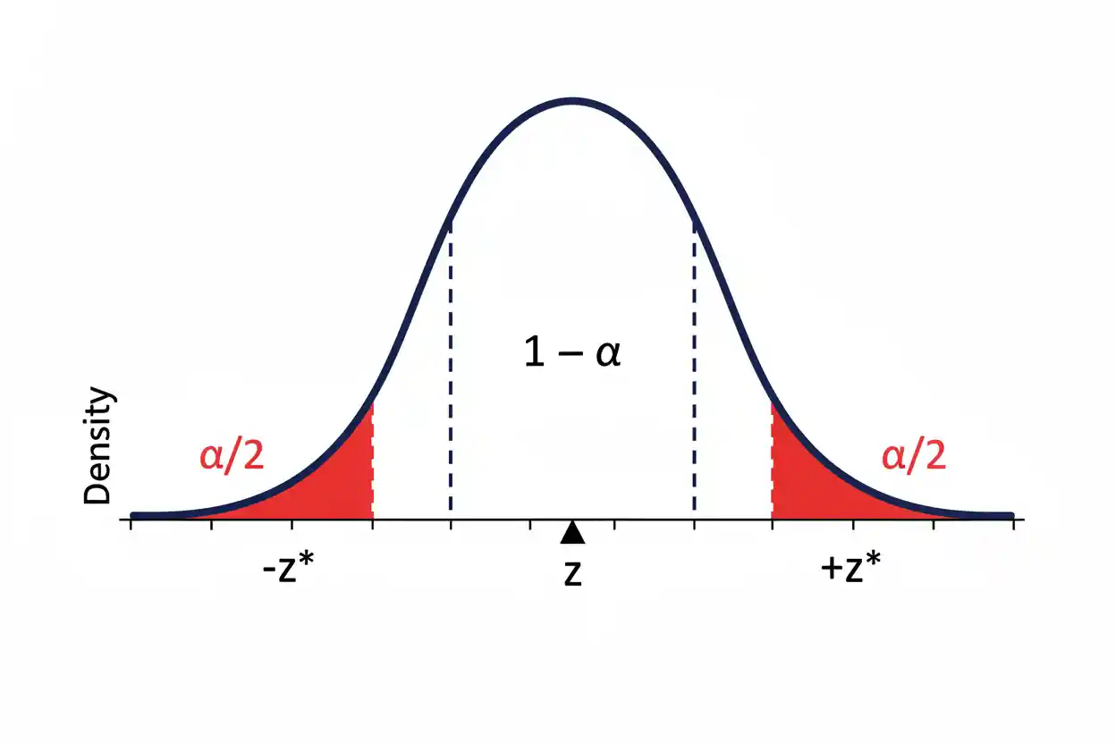

A critical value is a cutoff on a statistical reference distribution that separates results considered sufficiently extreme to reject a null hypothesis from results that do not cross the chosen rejection threshold. It is determined before interpreting the observed test statistic from factors such as the significance level, whether the test is one-tailed or two-tailed, the reference distribution, and—in distributions such as t, chi-square, and F—the appropriate degrees of freedom. For a two-sided standard normal test conducted at α = 0.05, for example, the familiar critical values are approximately −1.96 and +1.96 because 2.5% of the standard normal distribution lies beyond each cutoff. An observed z statistic greater than 1.96 or less than −1.96 therefore falls inside a rejection region for that particular test.
Critical values are also fundamental to confidence intervals because an estimate is commonly extended by a critical value multiplied by its standard error to construct a margin of error. They should not be confused with p-values, effect sizes, test statistics, or arbitrary benchmarks chosen after seeing the data. A critical value reflects the decision rule established by the inferential procedure, while the observed statistic describes what the sample actually produced. Understanding how these quantities interact makes hypothesis tests and confidence intervals considerably easier to interpret correctly.
Critical values are a foundational topic within Statistics & Probability and the broader Inference & Regression framework. They provide thresholds for inferential decisions, while related quantities such as effect size answer different questions about the magnitude of an observed difference or relationship.
What Is a Critical Value?
A critical value is a point on the probability distribution of a test statistic under the null hypothesis. It defines the boundary of a rejection region.
Suppose a test statistic T has a known reference distribution when H₀ is true. If the alternative hypothesis predicts unusually large values, the decision rule might take the form:
Reject H₀ if T > c
where c is the critical value.
For a two-sided test, there are usually two boundaries:
Reject H₀ if T < −c or T > c
when the reference distribution is symmetric around zero.
The value of c is chosen so that the probability of entering the rejection region when H₀ is true equals the selected significance level α.
Conceptually:
P(test statistic falls in rejection region | H₀) = α
A critical value is therefore not calculated from how convincing the sample “looks.” It follows from the probability model and decision threshold selected for the statistical procedure.
Critical Value and Significance Level
The significance level α determines how much probability is allocated to the rejection region under H₀.
Common choices include:
α = 0.10
α = 0.05
α = 0.01
If α = 0.05, the test procedure permits a 5% long-run probability of rejecting H₀ when H₀ is actually true, assuming the model and testing procedure are correctly specified.
The critical value is chosen to create that probability.
For a right-tailed standard normal test at α = 0.05:
P(Z > zcritical) = 0.05
The corresponding critical value is approximately:
zcritical ≈ 1.645
Therefore:
Reject H₀ if z > 1.645
For a smaller significance level such as α = 0.01, the rejection region must move farther into the tail. The right-tailed standard normal critical value then becomes approximately:
zcritical ≈ 2.326
A more demanding significance threshold therefore generally produces a more extreme critical value.
The Critical Value Is a Quantile
Mathematically, a critical value is a quantile of the reference distribution.
Let F represent the cumulative distribution function of a continuous test statistic under H₀. For a right-tailed test with significance level α:
c = F⁻¹(1 − α)
where F⁻¹ denotes the quantile function.
For a left-tailed test:
c = F⁻¹(α)
For a symmetric two-tailed test with total significance level α, the upper cutoff is:
c = F⁻¹(1 − α/2)
and the lower cutoff is:
−c
when symmetry applies.
These equations explain why there is no single universal critical value. The cutoff depends on both the chosen tail probability and the probability distribution used by the statistical procedure.
One-Tailed vs Two-Tailed Critical Values
Whether a hypothesis test is one-tailed or two-tailed has a direct effect on its critical value.
Consider α = 0.05 with a standard normal reference distribution.
For a right-tailed test, the entire 5% rejection probability is placed in the upper tail:
zcritical ≈ 1.645
Also, For a left-tailed test:
zcritical ≈ −1.645
For a two-tailed test, the 5% rejection probability is divided equally between two tails:
α/2 = 0.025
The critical values become:
zcritical ≈ ±1.96
Because each tail contains only 2.5%, the two-sided cutoffs must lie farther from zero than the one-sided 5% cutoff.
The direction of the test must follow the research hypothesis and be established independently of the observed data. Selecting a one-tailed test after seeing that the result moved in a favorable direction improperly changes the decision rule.
Standard Normal Critical Values
For tests based on the standard normal distribution, several critical values appear frequently.
| Significance Level | Test Type | Critical Value |
|---|---|---|
| α = 0.10 | Two-tailed | ±1.645 |
| α = 0.05 | Two-tailed | ±1.960 |
| α = 0.02 | Two-tailed | ±2.326 |
| α = 0.01 | Two-tailed | ±2.576 |
| α = 0.10 | One-tailed | ±1.282 |
| α = 0.05 | One-tailed | ±1.645 |
| α = 0.01 | One-tailed | ±2.326 |
The sign used in a one-tailed test depends on whether the rejection region is in the lower or upper tail.
For example, a right-tailed test at α = 0.05 uses:
+1.645
whereas a left-tailed test uses:
−1.645
These values are properties of the standard normal distribution rather than constants that apply to every hypothesis test.
Worked Example: Two-Tailed Z Test
Suppose a hypothesis test uses a standard normal test statistic and has:
α = 0.05
The alternative hypothesis is two-sided, so the significance level is divided equally between both tails:
α/2 = 0.025
The standard normal cutoff leaving 2.5% above it is:
zcritical ≈ 1.96
The two critical values are therefore:
−1.96 and +1.96
The decision rule is:
Reject H₀ if z < −1.96 or z > 1.96
Suppose the observed test statistic is:
z = 2.31
Because:
2.31 > 1.96
the test statistic falls inside the rejection region, so H₀ is rejected at α = 0.05.
If instead:
z = 1.70
then:
−1.96 < 1.70 < 1.96
so the statistic is not inside either rejection tail. The test fails to reject H₀ at that significance level.
The critical value therefore provides a direct cutoff-based decision rule.
Worked Example: One-Tailed Z Test
Suppose a researcher has a directional alternative and uses a right-tailed test with:
α = 0.05
The standard normal critical value is:
zcritical ≈ 1.645
The decision rule becomes:
Reject H₀ if z > 1.645
If:
zobserved = 1.82
then:
1.82 > 1.645
and H₀ is rejected.
Notice that 1.82 would not cross the two-tailed α = 0.05 cutoff of 1.96. This difference occurs because the one-sided procedure places all of the allowable Type I error probability in one tail.
A one-sided test should only be used when the directional hypothesis is substantively appropriate before examining the sample result.
Rejection Region
A rejection region is the set of test-statistic values beyond the relevant critical value or values.
For a right-tailed test:
Rejection region: T > c
Also, For a left-tailed test:
Rejection region: T < c
For a symmetric two-tailed test:
Rejection region: T < −c or T > c
The area of the rejection region under the null reference distribution equals α.
This gives the critical-value approach its long-run error-control interpretation. If H₀ were repeatedly true and the entire sampling procedure were repeated many times, the statistic would enter the predefined rejection region with probability α under the model assumptions.
The critical region is therefore a property of the test procedure—not a region of the original raw-data distribution.
Critical Value vs Test Statistic
A critical value and a test statistic have different roles.
The critical value comes from the theoretical reference distribution and selected significance level. The observed test statistic is calculated from the sample.
The decision compares them.
For a right-tailed test:
observed statistic > critical value → reject H₀
For a two-sided standardized test:
|observed statistic| > critical value → reject H₀
Suppose:
zcritical = 1.96
and:
zobserved = 2.40
Because:
|2.40| > 1.96
the observed statistic lies in the rejection region.
The value 1.96 says nothing about the magnitude of the underlying real-world effect by itself. It is simply the cutoff generated by the selected inferential procedure.
Critical Value vs P-Value
The critical-value approach and p-value approach are two equivalent ways to make the same hypothesis-test decision when they are based on the same statistical model and significance level.
Using the critical-value approach:
Reject H₀ if test statistic falls beyond the critical value.
Using the p-value approach:
Reject H₀ if p-value < α.
Suppose a two-sided z test uses:
α = 0.05
so:
zcritical = ±1.96
If the observed result is:
z = 2.20
then it exceeds the critical boundary. The corresponding two-sided p-value is also below 0.05, so both approaches reject H₀.
The p-value contains additional information about how far into the tail the observed statistic lies. A critical-value comparison supplies the binary decision for the selected α.
Neither quantity is the probability that H₀ is true.
Why Critical Values Change With α
Critical values become more extreme when α decreases because a smaller rejection region must be placed farther into the tails of the reference distribution.
For a two-sided standard normal test:
α = 0.10 → zcritical ≈ ±1.645
α = 0.05 → zcritical ≈ ±1.960
α = 0.01 → zcritical ≈ ±2.576
At α = 0.01, an observed result must be farther from the center of the null distribution to qualify for rejection than at α = 0.05.
This reduces the probability of a Type I error but, all else equal, can make it harder to detect a genuine effect. Inferential thresholds therefore involve tradeoffs rather than a universal significance level that is optimal for every decision.
Critical Values for the t Distribution
When a test statistic follows Student’s t distribution rather than the standard normal distribution, the critical value depends on the degrees of freedom as well as α and the tail structure.
For a two-tailed test:
tcritical = t₁₋α/₂,df
The t distribution has heavier tails than the standard normal distribution, especially with few degrees of freedom. Therefore, its two-sided critical values are generally larger in magnitude than 1.96 at α = 0.05 when df is finite.
For example, with:
df = 19
and:
α = 0.05
for a two-sided test:
tcritical ≈ ±2.093
With many more degrees of freedom, the t distribution approaches the standard normal distribution, so the critical value gradually approaches:
±1.96
This is why sample size or, more precisely, degrees of freedom can affect a t critical value even when α remains unchanged.
Worked Example With a t Critical Value
Suppose a two-sided t test has:
df = 19
α = 0.05
The appropriate cutoff is approximately:
tcritical = ±2.093
Suppose the calculated statistic is:
tobserved = 2.35
Because:
|2.35| > 2.093
the test statistic enters the rejection region.
If instead:
tobserved = 1.90
then:
|1.90| < 2.093
and H₀ is not rejected at α = 0.05.
The same observed statistic could produce a different decision with different degrees of freedom because the t reference distribution changes as df changes.
Degrees of Freedom Matter
Degrees of freedom determine the shape of several reference distributions used in inferential statistics. Consequently, they can materially change the critical value.
For Student’s t distribution, smaller df produce heavier tails and more extreme critical values.
Also, For chi-square distributions, changing df alters both the center and shape of the distribution.
For F distributions, the critical value depends on two sets of degrees of freedom.
There is therefore no meaningful instruction to “use the 0.05 critical value” without also identifying the statistical distribution and any required degrees of freedom.
The complete specification is more like:
two-sided t critical value at α = 0.05 with df = 19
or:
upper-tail chi-square critical value at α = 0.05 with df = 4
Chi-Square Critical Values
The chi-square distribution is generally right-skewed and nonnegative. For many chi-square hypothesis tests, evidence against H₀ lies in the upper tail, so the decision rule takes the form:
Reject H₀ if χ²observed > χ²critical
The critical value depends on both α and df.
For example, the chi-square test of independence uses a chi-square reference distribution whose degrees of freedom are determined by the dimensions of the contingency table. Once df and α are known, the corresponding upper-tail critical value can be obtained.
This illustrates why a critical value is not tied exclusively to z or t procedures. The same general idea applies across multiple inferential distributions, even though the numerical cutoffs and tail structures differ.
F Critical Values
F distributions are used in several inferential settings involving ratios of variance-like quantities. An F critical value depends on:
α
numerator degrees of freedom
denominator degrees of freedom
A typical upper-tail rule takes the form:
Reject H₀ if Fobserved > Fcritical
Because an F distribution is asymmetric and defined for nonnegative values, its critical values behave differently from the symmetric ±z or ±t cutoffs often encountered in two-sided standardized tests.
This reinforces the general principle that the phrase “critical value” describes the role of a threshold, not one particular numerical value or probability distribution.
Critical Values and Confidence Intervals
Critical values also determine the width of many confidence intervals.
A common interval structure is:
estimate ± critical value × standard error
The quantity:
critical value × standard error
is the margin of error.
For a large-sample normal-based 95% interval, the critical value is approximately:
z* = 1.96
So the interval has the form:
estimate ± 1.96 × SE
For a 99% normal-based interval:
z* ≈ 2.576
The higher confidence level requires a larger critical value, producing a wider interval when the standard error is unchanged.
A wider interval reflects the tradeoff required to achieve greater long-run coverage.
Worked Confidence Interval Example
Suppose an estimate is:
50
with standard error:
SE = 4
For a normal-based 95% interval:
critical value = 1.96
The margin of error is:
ME = 1.96 × 4
ME = 7.84
Therefore:
Lower bound = 50 − 7.84 = 42.16
Upper bound = 50 + 7.84 = 57.84
The interval is:
42.16 to 57.84
For a 99% interval using:
z* ≈ 2.576
the margin of error becomes:
ME = 2.576 × 4
ME = 10.304
giving:
39.696 to 60.304
The higher confidence level produces a wider interval because its critical value is larger.
Confidence Level and Critical Value
For the familiar two-sided normal interval:
Confidence level = 1 − α
A 95% confidence level corresponds to:
α = 0.05
and places:
α/2 = 0.025
in each tail.
This gives:
z* ≈ 1.96
A 90% interval leaves:
α = 0.10
or 5% in each tail, producing:
z* ≈ 1.645
A 99% interval leaves only 0.5% in each tail and therefore uses:
z* ≈ 2.576
Greater confidence requires covering a larger portion of the reference distribution, so the cutoff moves farther into the tails.
Critical Value Is Not an Effect Size
A critical value should not be interpreted as the magnitude of the phenomenon being studied.
Suppose:
zcritical = 1.96
This does not mean the effect has a standardized magnitude of 1.96.
A measure such as Cohen D is designed to describe a standardized mean difference. A critical value instead marks a threshold on a test statistic’s reference distribution.
The two values can appear in the same analysis but answer completely different questions.
Statistical significance concerns whether evidence crosses an inferential threshold. Practical importance concerns the magnitude and consequences of an effect. One should not substitute for the other.
Critical Value vs Coefficient of Determination
The coefficient of determination, R², measures regression fit relative to a baseline under its conventional interpretation. It does not serve as a rejection threshold.
A result such as:
R² = 0.70
does not imply a critical value of 0.70.
Likewise:
zcritical = 1.96
does not mean that a regression model accounts for 196% of variation.
Critical values belong to inferential decision rules. R² belongs to model-fit interpretation. Keeping these roles separate prevents numerical quantities from being given meanings they do not possess.
Critical Values in Regression
Critical values also appear in inferential procedures for regression coefficients. Suppose a regression coefficient estimate is divided by its standard error to produce a test statistic. That statistic can then be compared with an appropriate critical value from its reference distribution.
Conceptually:
test statistic = estimate / standard error
under a null hypothesis in which the tested coefficient is zero, with the exact form depending on the model.
If:
|test statistic| > critical value
for a two-sided procedure, H₀ may be rejected at the specified α.
The exact distribution and degrees of freedom depend on the regression method. For example, inferential procedures associated with logistic regression can use large-sample standardized statistics, but the interpretation and assumptions belong to that model rather than to the general definition of critical values.
Choosing α Before Looking at the Result
The significance threshold should be selected according to the research context and decision consequences rather than adjusted to make an observed result cross a preferred boundary.
Suppose a study initially specifies:
α = 0.01
but produces a two-sided z statistic:
z = 2.10
The statistic exceeds the α = 0.05 critical value:
1.96
but does not exceed the α = 0.01 cutoff:
2.576
Changing α from 0.01 to 0.05 after seeing the result simply to obtain rejection undermines the meaning of the prespecified error rate.
A threshold should reflect how costly false positives and false negatives are, relevant conventions, and the broader decision environment.
Critical Values and Type I Error
A Type I error occurs when H₀ is rejected even though it is true.
The significance level determines the probability of this event under the test’s assumptions:
P(Type I error | H₀ true) = α
Critical values implement this error threshold geometrically on the reference distribution.
For a two-sided standard normal test at α = 0.05, the rejection regions beyond ±1.96 jointly contain 5% of the probability under H₀.
That does not mean there is a 5% probability that H₀ is true after an observed statistic crosses the threshold. The 5% refers to the procedure’s behavior when H₀ is assumed true.
Critical Values and Statistical Power
Moving a critical value farther into the tail can reduce the probability of a Type I error but, all else equal, may also make genuine departures from H₀ harder to detect.
For example, compare two right-tailed standard normal tests:
α = 0.05 → zcritical ≈ 1.645
α = 0.01 → zcritical ≈ 2.326
A true effect must generally produce a more extreme test statistic to cross the second boundary.
This relationship connects the significance level with statistical power. The appropriate balance depends on the consequences of false positive and false negative conclusions rather than on an automatic preference for the smallest possible α.
Critical Values and Sample Size
For a z test, the standard normal critical value at a fixed α does not change merely because sample size changes. A two-sided α = 0.05 z procedure continues to use:
±1.96
However, sample size affects the standard error and therefore can affect the observed standardized test statistic.
For t procedures, sample size can also affect the critical value indirectly through the degrees of freedom. As df increases, the t critical value moves closer to the corresponding normal critical value.
Thus, sample size and critical value should not be conflated. Their relationship depends on the reference distribution being used.
Why 1.96 Is So Common
The value 1.96 appears frequently because it is the standard normal cutoff associated with a central probability of approximately 95%.
Specifically:
P(−1.96 ≤ Z ≤ 1.96) ≈ 0.95
leaving approximately:
0.025
in each tail.
Therefore, ±1.96 is used for a two-sided standard normal hypothesis test with α = 0.05 and for many normal-based 95% confidence intervals.
It is not a universal statistical cutoff. A one-sided 5% test uses 1.645, a 99% two-sided procedure uses approximately 2.576, and t, chi-square, and F procedures use different cutoffs.
How to Find a Critical Value
The general process begins by identifying the statistical procedure and its reference distribution. Determine whether the relevant statistic follows a z, t, chi-square, F, or another distribution under H₀.
Next identify the significance level:
α
Then determine whether the test is:
left-tailed
right-tailed
or:
two-tailed
For distributions requiring degrees of freedom, calculate the appropriate df. Finally, obtain the quantile that leaves the required probability in the rejection tail or tails.
For a symmetric two-tailed test:
upper-tail probability = α/2
For a one-tailed test:
tail probability = α
The resulting quantile is the critical value.
Example: Finding a Z Critical Value
Suppose:
α = 0.05
and the test is two-tailed.
Divide the total significance level between the two tails:
α/2 = 0.025
The cumulative probability to the left of the upper critical value is:
1 − 0.025 = 0.975
The 97.5th percentile of the standard normal distribution is approximately:
1.96
Therefore:
critical values = −1.96 and +1.96
This procedure explains the number rather than requiring it to be memorized.
Example: Finding a One-Sided Critical Value
Suppose:
α = 0.01
for a right-tailed standard normal test.
The cumulative probability below the cutoff must be:
1 − 0.01 = 0.99
The 99th percentile of the standard normal distribution is approximately:
2.326
Therefore:
zcritical ≈ 2.326
and the rejection rule is:
Reject H₀ if z > 2.326
For a left-tailed test at the same α, symmetry gives:
zcritical ≈ −2.326
Common Mistakes
A common mistake is treating 1.96 as the critical value for every statistical test. It is only one particular standard normal cutoff.
Another error is forgetting to divide α between the tails in a two-sided procedure. Using 1.645 rather than 1.96 for a two-sided α = 0.05 z test changes the Type I error rate.
Researchers can also confuse the critical value with the observed statistic. The critical value comes from the reference distribution; the test statistic comes from the sample.
Another mistake is interpreting crossing a critical value as proof that the alternative hypothesis is true. A rejection decision is an inferential conclusion made under uncertainty and remains subject to the specified Type I error rate and model assumptions.
Finally, statistical significance should not be interpreted as practical importance. Crossing a threshold says that an observed statistic is sufficiently extreme under H₀; it does not indicate how consequential the underlying effect is.
Critical Value Decision Checklist
First identify H₀ and H₁ clearly. Determine whether the alternative requires a lower-tail, upper-tail, or two-tail rejection region. Select α according to the analysis plan and consequences of errors rather than according to the observed result.
Next identify the null reference distribution and any required degrees of freedom. Use those inputs to obtain the appropriate critical value. Then calculate the observed test statistic independently from the sample.
Finally compare the observed statistic with the rejection boundary. If it crosses the critical value in the direction specified by the test, reject H₀. Otherwise, fail to reject H₀.
The conclusion should be expressed in the context of the original research question without turning a threshold-based statistical decision into a claim of certainty.
Frequently Asked Questions
What is a critical value in statistics?
A critical value is a cutoff on the null distribution of a test statistic. Values beyond that cutoff belong to a rejection region for the selected significance level.
What determines a critical value?
It depends on the reference distribution, significance level, one-tailed or two-tailed structure, and any required degrees of freedom.
What is the critical value for α = 0.05?
There is no single answer without specifying the statistical procedure. For a standard normal test, it is approximately 1.645 for a one-tailed test and ±1.96 for a two-tailed test.
Why is 1.96 a critical value?
For a standard normal distribution:
P(−1.96 ≤ Z ≤ 1.96) ≈ 0.95
so approximately 2.5% remains in each tail. This corresponds to a two-sided α = 0.05 procedure.
What is the difference between a critical value and a test statistic?
The critical value is the theoretical rejection cutoff. The test statistic is calculated from the observed sample and compared with that cutoff.
What is the difference between a critical value and a p-value?
A critical value specifies the test-statistic boundary corresponding to α. A p-value indicates how extreme the observed statistic is under H₀. Both produce the same reject/fail-to-reject decision when based on the same test and α.
Does a critical value depend on sample size?
Sometimes indirectly. Standard normal critical values do not change with sample size at fixed α, while t critical values change as degrees of freedom change.
Why do t critical values depend on degrees of freedom?
Student’s t distributions have heavier tails when degrees of freedom are small. More extreme cutoffs are therefore needed to leave the same probability in the tails.
Is a larger critical value always better?
No. A larger cutoff makes rejection more difficult. Whether that tradeoff is appropriate depends on the chosen error rate and decision context.
Can a critical value be negative?
Yes. Left-tail critical values for symmetric distributions such as the standard normal can be negative. A two-sided test commonly has one negative and one positive critical value.
Can there be two critical values?
Yes. Two-sided tests generally have lower and upper critical values because extreme results in either direction can lead to rejection.
Is the critical value the same as effect size?
No. A critical value defines a hypothesis-test boundary. An effect-size statistic measures the magnitude of a difference or relationship.
How is a critical value used in a confidence interval?
Many confidence intervals use:
estimate ± critical value × standard error
The critical value determines how many standard errors extend from the estimate.
Why does a 99% confidence interval use a larger critical value than a 95% interval?
A 99% interval must cover more of the reference distribution, so its boundaries extend farther into the tails. With the same standard error, this produces a wider interval.
Does crossing a critical value prove H₁ is true?
No. It means the observed statistic lies in the predefined rejection region under H₀. Statistical testing does not convert uncertain evidence into mathematical proof of the alternative hypothesis.
Key Takeaway
A critical value is the boundary that defines a rejection region on the null distribution of a statistical test. It is determined from the reference distribution, significance level, tail structure, and—when applicable—degrees of freedom.
For a right-tailed procedure:
c = F⁻¹(1 − α)
For a symmetric two-tailed procedure, the upper cutoff is:
c = F⁻¹(1 − α/2)
with a corresponding lower cutoff in the opposite tail.
For the standard normal distribution, familiar examples include:
α = 0.05 one-tailed → zcritical ≈ 1.645
α = 0.05 two-tailed → zcritical ≈ ±1.96
α = 0.01 two-tailed → zcritical ≈ ±2.576
The critical value comes from the inferential procedure, while the observed test statistic comes from the sample. Crossing the relevant boundary leads to rejection of H₀ at the selected significance level; failing to cross it leads to failure to reject H₀. The value does not measure effect magnitude, practical importance, or the probability that a hypothesis is true. Its role is precise: it translates a chosen tail probability into the cutoff used for a statistical decision.



