
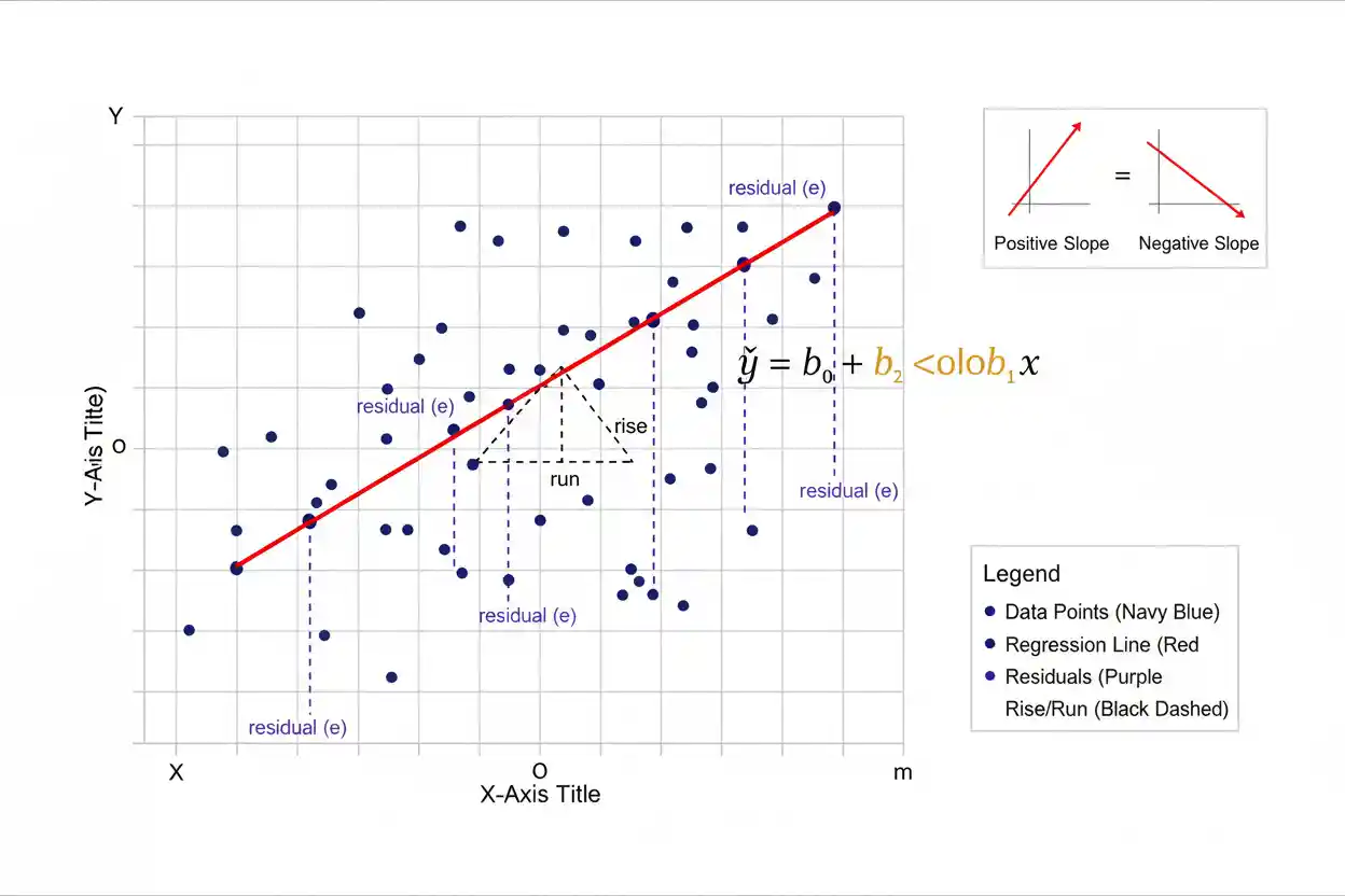

The regression slope is the coefficient that describes how the fitted response changes as a predictor changes. In simple linear regression, the equation is ŷ = b₀ + b₁x, where b₁ is the estimated slope and b₀ is the Regression Intercept. A positive slope means the fitted response increases as the predictor increases, while a negative slope means the fitted response decreases. A slope of zero produces a horizontal fitted line and indicates no estimated linear change in the response as x changes. The magnitude of the slope is expressed in response units per predictor unit, so its practical meaning depends directly on the measurement scales involved. Ordinary least squares estimates the slope by relating the joint variation of X and Y to the variation in X, choosing the line that minimizes the squared Residuals.
The estimated slope is a sample statistic rather than a known population quantity, so it has sampling uncertainty that can be described with a standard error, confidence interval, and hypothesis test. A statistically significant slope does not automatically imply a large effect, useful prediction, or causal relationship. Correct interpretation therefore requires attention to units, model specification, uncertainty, functional form, predictor range, influential observations, and the purpose for which the regression is being used.
Regression slope is a foundational topic in Statistics & Probability and Inference & Regression. It represents the rate of change encoded by a fitted regression model rather than merely the visual steepness of a line.
What Is a Regression Slope?
In simple linear regression:
ŷ = b₀ + b₁x
the regression slope is:
b₁
It measures the estimated change in the fitted value ŷ associated with a one-unit increase in x.
Suppose:
ŷ = 20 + 4x
Then:
b₁ = 4
A one-unit increase in x is associated with an estimated increase of four units in the fitted response.
If x rises from:
5 to 6
the predicted response rises by:
4(6 − 5) = 4
If x rises by ten units:
Change in ŷ = 4 × 10 = 40
The slope therefore describes a constant fitted rate of change in the basic simple linear model.
Regression Slope Formula
For ordinary least squares simple linear regression:
b₁ = Σ[(xᵢ − x̄)(yᵢ − ȳ)] / Σ(xᵢ − x̄)²
The numerator measures how X and Y vary together:
Σ[(xᵢ − x̄)(yᵢ − ȳ)]
The denominator measures variation in X:
Σ(xᵢ − x̄)²
Another common notation defines:
Sxy = Σ[(xᵢ − x̄)(yᵢ − ȳ)]
and:
Sxx = Σ(xᵢ − x̄)²
so:
b₁ = Sxy / Sxx
Once b₁ is known, the intercept can be calculated as:
b₀ = ȳ − b₁x̄
The fitted equation is then:
ŷ = b₀ + b₁x
Why This Formula Produces the Slope
The slope compares how much X and Y move together with how much X itself varies.
If values above x̄ tend to occur with values above ȳ, while values below x̄ tend to occur with values below ȳ, the cross-products:
(xᵢ − x̄)(yᵢ − ȳ)
are mostly positive.
This produces:
b₁ > 0
If values above x̄ tend to occur with values below ȳ, the cross-products tend to be negative, producing:
b₁ < 0
If there is little systematic linear co-movement, positive and negative cross-products can largely offset one another and the slope may be near zero.
The denominator rescales this joint variation according to the spread of X.
Worked Regression Slope Example
Suppose the following observations are available:
| x | y |
|---|---|
| 1 | 2 |
| 2 | 4 |
| 3 | 5 |
| 4 | 8 |
| 5 | 11 |
First calculate the means:
x̄ = (1 + 2 + 3 + 4 + 5) / 5
x̄ = 3
and:
ȳ = (2 + 4 + 5 + 8 + 11) / 5
ȳ = 6
Now calculate:
Sxy = Σ[(xᵢ − 3)(yᵢ − 6)]
The individual products are:
(1 − 3)(2 − 6) = 8
(2 − 3)(4 − 6) = 2
(3 − 3)(5 − 6) = 0
(4 − 3)(8 − 6) = 2
(5 − 3)(11 − 6) = 10
Therefore:
Sxy = 8 + 2 + 0 + 2 + 10
Sxy = 22
Now calculate:
Sxx = Σ(xᵢ − 3)²
= 4 + 1 + 0 + 1 + 4
= 10
The estimated slope is:
b₁ = 22 / 10
b₁ = 2.2
The fitted response therefore increases by approximately 2.2 units for every one-unit increase in x.
Calculate the Intercept
Using:
b₀ = ȳ − b₁x̄
substitute:
ȳ = 6
b₁ = 2.2
x̄ = 3
Then:
b₀ = 6 − 2.2(3)
b₀ = 6 − 6.6
b₀ = −0.6
The fitted regression equation is:
ŷ = −0.6 + 2.2x
At:
x = 4
the predicted response is:
ŷ = −0.6 + 2.2(4)
ŷ = −0.6 + 8.8
ŷ = 8.2
The observed response at x = 4 is 8, so the corresponding residual is:
e = y − ŷ
e = 8 − 8.2
e = −0.2
How to Interpret the Regression Slope
A useful slope interpretation should always state both the change in the predictor and the expected or fitted change in the response.
For:
ŷ = −0.6 + 2.2x
a correct interpretation is:
For each one-unit increase in x, the fitted value of y increases by approximately 2.2 units.
If x represents hours of study and y represents examination points:
Each additional study hour is associated with an estimated 2.2-point increase in the fitted examination score.
The phrase “associated with” is usually appropriate for observational regression because a slope alone does not establish a causal effect.
Units of the Regression Slope
The slope has units:
units of Y / units of X
Suppose Y is measured in dollars and X in hours.
If:
b₁ = 25
then the slope is:
25 dollars per hour
If Y is kilograms and X is meters:
slope units = kilograms per meter
This means slope magnitude cannot be compared meaningfully across arbitrary measurement scales without considering the units.
A slope of 100 is not inherently “stronger” than a slope of 0.5. One may simply use much smaller measurement units than the other.
Positive Regression Slope
A positive slope means:
b₁ > 0
As x increases, the fitted value of y increases.
For example:
ŷ = 15 + 3x
has:
b₁ = 3
If x increases by five units:
Change in ŷ = 3 × 5
Change in ŷ = 15
The regression line rises from left to right.
A positive slope describes a positive linear association in the fitted model. It does not automatically establish that increasing X will cause Y to increase.
Negative Regression Slope
A negative slope means:
b₁ < 0
For example:
ŷ = 100 − 4x
has:
b₁ = −4
A one-unit increase in x is associated with an estimated four-unit decrease in the response.
If x rises by:
10 units
then:
Change in ŷ = −4(10)
Change in ŷ = −40
Graphically, the fitted line falls from left to right.
The negative sign describes direction rather than statistical importance.
Zero Regression Slope
If:
b₁ = 0
then:
ŷ = b₀
The fitted value is constant regardless of x.
The regression line is horizontal.
This represents no estimated linear relationship between X and Y in a simple linear regression.
However, a zero slope does not necessarily mean X and Y are completely unrelated. A strong nonlinear relationship can exist while the best-fitting linear slope is zero or approximately zero.
For example, a symmetric U-shaped relationship may have substantial dependence but little overall linear trend.
Population Slope vs Sample Slope
The population regression model is:
Y = β₀ + β₁X + ε
The population slope is:
β₁
A sample is used to estimate it with:
b₁
Therefore:
β₁ = population parameter
while:
b₁ = sample statistic
Different random samples from the same population generally produce different b₁ values.
This sampling variability means the observed slope should not be treated as the exact population relationship.
Statistical inference is used to quantify how uncertain the estimate is.
Regression Slope and Ordinary Least Squares
Ordinary least squares chooses the intercept and slope that minimize:
SSE = Σ(yᵢ − ŷᵢ)²
For simple regression:
ŷᵢ = b₀ + b₁xᵢ
so:
SSE = Σ[yᵢ − (b₀ + b₁xᵢ)]²
The slope is therefore not chosen simply by drawing a visually plausible line.
It is the coefficient belonging to the line with the smallest possible sum of squared residuals among all lines of the specified form.
The squared-error criterion gives larger residuals disproportionately more numerical influence because their errors are squared.
Regression Slope and Residuals
The Residuals are:
eᵢ = yᵢ − ŷᵢ
The slope determines how the fitted values change across X, so it directly affects the residual pattern.
If the slope is too low, predictions may systematically overestimate Y at low X values and underestimate Y at high X values.
If the slope is too high, the opposite pattern can occur.
OLS selects b₁ jointly with b₀ so that the resulting squared residual total is minimized.
Residual analysis then helps determine whether a straight-line slope is an adequate representation of the relationship.
Regression Slope and Covariance
The sample covariance can be written:
sxy = Σ[(xᵢ − x̄)(yᵢ − ȳ)] / (n − 1)
The sample variance of X is:
sx² = Σ(xᵢ − x̄)² / (n − 1)
Dividing covariance by variance gives:
b₁ = sxy / sx²
because the common:
n − 1
terms cancel.
This provides another useful interpretation:
regression slope = covariance of X and Y / variance of X
The slope therefore depends on both how strongly the variables co-vary and the scale of the predictor.
Regression Slope and Correlation
The sample correlation is:
r = sxy / (sxsy)
Rearranging gives:
sxy = r sx sy
Substitute this into:
b₁ = sxy / sx²
to obtain:
b₁ = r(sy / sx)
Thus, in simple linear regression:
b₁ = r × sy / sx
This shows why the slope and correlation always have the same sign in ordinary simple regression.
If:
r > 0
then:
b₁ > 0
If:
r < 0
then:
b₁ < 0
If:
r = 0
then:
b₁ = 0
provided sx is nonzero.
Slope Is Not the Same as Correlation
Although slope and correlation are related, they measure different things.
Correlation is unitless and generally lies between:
−1 and +1
The slope has units and can take any real value.
Suppose:
r = 0.8
This does not imply:
b₁ = 0.8
Instead:
b₁ = 0.8 × sy / sx
If:
sy / sx = 10
then:
b₁ = 8
The relationship between slope and correlation therefore depends on the relative standard deviations of the two variables.
Effect of Changing X Units
Suppose a predictor is originally measured in meters and the fitted model is:
ŷ = 10 + 5xmeters
The slope is:
5 response units per meter
Now measure X in centimeters.
Since:
1 meter = 100 centimeters
a one-centimeter increase is only 1/100 of a meter.
The equivalent slope becomes:
5 / 100
0.05 response units per centimeter
The fitted relationship has not changed. Only the numerical representation of the slope changed because the predictor units changed.
This demonstrates why raw slopes should always be interpreted with units.
Effect of Changing Y Units
Suppose Y is measured in dollars and:
b₁ = 20 dollars per unit of X
If Y is converted to cents:
1 dollar = 100 cents
the slope becomes:
2,000 cents per unit of X
Again, the underlying relationship is identical.
The coefficient changes because the response scale changes.
A numerically larger slope therefore does not necessarily represent a larger substantive relationship.
Centering X Does Not Change the Simple Regression Slope
Suppose:
xc = x − c
where c is a constant.
An original model:
ŷ = b₀ + b₁x
can be rewritten:
ŷ = b₀ + b₁(xc + c)
ŷ = (b₀ + b₁c) + b₁xc
The intercept changes, but the slope remains:
b₁
Therefore, subtracting a constant from X changes where zero is located but does not change the simple regression slope.
This is why centering is often used to make the intercept easier to interpret without changing the fitted rate of change.
Standardized Regression Slope
If both X and Y are standardized to mean zero and standard deviation one, the simple regression slope becomes:
b₁,standardized = r
This follows from:
b₁ = r(sy / sx)
because after standardization:
sx = 1
and:
sy = 1
so:
b₁ = r
In multiple regression, standardized coefficients do not generally equal simple pairwise correlations because each slope is conditional on the other included predictors.
Standardization can help compare coefficients expressed on different scales, but it does not automatically reveal causal or practical importance.
Regression Slope in Multiple Regression
A multiple linear regression is:
ŷ = b₀ + b₁x₁ + b₂x₂ + … + bₖxₖ
Each slope has a conditional interpretation.
For example:
b₁
represents the estimated change in ŷ associated with a one-unit increase in x₁ while holding the other included predictors constant.
Suppose:
ŷ = 50 + 3x₁ − 2x₂
Then:
b₁ = 3
means a one-unit increase in x₁ is associated with a three-unit increase in the fitted response when x₂ remains fixed.
Meanwhile:
b₂ = −2
means a one-unit increase in x₂ is associated with a two-unit decrease in the fitted response when x₁ remains fixed.
These are partial regression slopes.
Why a Slope Can Change When Predictors Are Added
Suppose a simple regression produces:
b₁ = 8
for the relationship between X₁ and Y.
After X₂ is added:
b₁ = 3
This does not necessarily mean one of the estimates is incorrect.
The interpretation has changed.
The simple-regression slope describes the overall linear association between X₁ and Y.
The multiple-regression slope describes the relationship between X₁ and Y conditional on the other included predictors.
If X₁ and X₂ are related, adjustment can substantially change the estimated coefficient.
A regression slope therefore belongs to a particular model specification.
Interaction Terms Change Slope Interpretation
Consider:
ŷ = b₀ + b₁x₁ + b₂x₂ + b₃x₁x₂
The slope with respect to x₁ is:
Change in ŷ per unit of x₁ = b₁ + b₃x₂
The slope of x₁ therefore depends on x₂.
There is no single constant effect of x₁ across all values of x₂ when:
b₃ ≠ 0
In this model, b₁ is specifically the slope of x₁ when:
x₂ = 0
This is one reason centering interacting predictors around meaningful values can improve interpretation.
Nonlinear Models and Local Slopes
A polynomial regression may contain:
ŷ = b₀ + b₁x + b₂x²
This model does not have one constant rate of change across X.
The derivative is:
dŷ/dx = b₁ + 2b₂x
so the local slope changes with x.
The coefficient b₁ alone should therefore not be described as the universal slope of the fitted curve.
It represents the local slope at:
x = 0
within the quadratic model.
This distinction prevents slope interpretations from a simple straight-line model being carried incorrectly into nonlinear specifications.
Standard Error of the Regression Slope
In simple OLS regression under the usual constant-variance framework, the estimated standard error of the slope is:
SE(b₁) = sₑ / √Sxx
where:
Sxx = Σ(xᵢ − x̄)²
and sₑ is the residual standard error.
This formula shows two important influences on slope precision.
First, greater unexplained residual variability increases:
sₑ
and therefore increases slope uncertainty.
Second, greater spread in the observed x-values increases:
Sxx
and therefore reduces the standard error of b₁, other factors held constant.
A well-spread predictor can provide more information about a rate of change than the same number of observations concentrated in a very narrow x-range.
Sampling Distribution of the Slope
Because b₁ is calculated from a random sample, it has a Sampling Distribution.
Across repeated samples from the same population and under the same model:
b₁
will vary from sample to sample.
Under the classical normal-error simple regression model:
(b₁ − β₁) / SE(b₁)
follows the relevant Student’s t distribution when the standard error is estimated in the usual way.
This sampling behavior provides the basis for confidence intervals and hypothesis tests concerning β₁.
The observed slope should therefore be interpreted as an estimate with uncertainty rather than a fixed known population relationship.
Testing a Regression Slope
A common null hypothesis is:
H₀: β₁ = 0
with a two-sided alternative:
H₁: β₁ ≠ 0
The test statistic is:
t = b₁ / SE(b₁)
More generally, for a hypothesized slope β₁,0:
t = (b₁ − β₁,0) / SE(b₁)
In simple linear regression with an intercept:
df = n − 2
because two parameters are estimated:
β₀ and β₁
A sufficiently large absolute t statistic provides evidence against the stated null slope under the model assumptions.
Worked Slope Hypothesis Test
Suppose:
b₁ = 2.4
and:
SE(b₁) = 0.8
Test:
H₀: β₁ = 0
The statistic is:
t = 2.4 / 0.8
t = 3
Suppose:
n = 22
Then:
df = 22 − 2
df = 20
For a two-sided test, a t statistic of 3 with 20 degrees of freedom corresponds to a p-value below 0.01.
The data therefore provide evidence that the population linear slope differs from zero under the model assumptions.
This conclusion concerns statistical evidence about β₁. It does not establish causation or practical importance.
Confidence Interval for the Regression Slope
A conventional confidence interval for the population slope is:
b₁ ± t* × SE(b₁)
Suppose:
b₁ = 2.4
SE(b₁) = 0.8
and:
t* ≈ 2.086
for a 95% interval with 20 degrees of freedom.
The margin of error is:
2.086 × 0.8
≈ 1.669
Therefore:
Lower ≈ 2.4 − 1.669
Lower ≈ 0.731
and:
Upper ≈ 2.4 + 1.669
Upper ≈ 4.069
The approximate 95% confidence interval is:
0.73 to 4.07
Zero is excluded, consistent with rejecting H₀: β₁ = 0 using the corresponding two-sided 5% test.
Confidence Interval vs Prediction Interval
A confidence interval for β₁ describes uncertainty about the population slope.
A Prediction Interval describes uncertainty about a future response.
These are different statistical targets.
A slope can be estimated very precisely while prediction intervals remain wide because individual observations vary considerably around the regression line.
Suppose:
β₁ is clearly positive
but residual variability is very large.
The model can provide strong evidence about the direction of the average relationship while still predicting individual Y values imprecisely.
Parameter precision and prediction precision should therefore not be confused.
Statistical Significance vs Slope Magnitude
A slope can be very small but statistically significant when estimated from a large, precise dataset.
Suppose:
b₁ = 0.01
with:
SE(b₁) = 0.001
Then:
t = 10
The evidence against β₁ = 0 is extremely strong.
Yet a change of 0.01 response units per predictor unit may be practically trivial.
Conversely:
b₁ = 10
with:
SE(b₁) = 8
produces:
t = 1.25
The observed slope is much larger numerically but far less precise.
Statistical evidence and effect magnitude must therefore be interpreted separately.
Slope and Predictor Range
Suppose:
b₁ = 0.2
At first glance, the slope may appear small.
But if X commonly changes by:
500 units
the fitted response difference over that range is:
0.2 × 500
100
The practical meaning of a slope depends not only on its one-unit value but also on realistic predictor changes.
A one-unit interpretation can sometimes be unhelpful when one predictor unit is tiny.
In such cases, interpreting a 10-unit, 100-unit, or one-standard-deviation change may provide better context while preserving the same fitted model.
Interpolation and Slope Interpretation
The estimated slope is primarily supported by the predictor range represented in the data.
Suppose the observations cover:
10 ≤ x ≤ 40
The slope estimates the fitted relationship across that region.
Using it to predict changes between:
x = 500 and x = 501
assumes the same linear relationship extends far beyond the evidence.
That assumption may fail because of saturation, thresholds, physical constraints, market changes, or other nonlinear mechanisms.
A fitted slope is not automatically a universal rate valid over every conceivable predictor value.
Outliers and Influential Observations
The OLS slope can be sensitive to unusual observations, especially points with extreme predictor values.
A point far from x̄ has high leverage and can strongly affect the orientation of the fitted line.
An observation may therefore shift b₁ substantially even if the rest of the data show a different pattern.
Influence should be assessed carefully rather than assuming every mathematically valid slope represents the dominant data structure.
Legitimate unusual observations should not be deleted simply because they weaken a preferred relationship.
Instead, analysts should investigate data quality, model suitability, and sensitivity of the estimated slope.
Restricted Predictor Range
If X varies only within a narrow interval, the slope can be estimated imprecisely because:
Sxx = Σ(xᵢ − x̄)²
is small.
Suppose all observed x-values lie between:
99 and 101
There is little information about how Y changes across a broad range of X.
A wider, relevant predictor range can improve slope precision, although deliberately increasing range must still respect the actual target population and experimental design.
Range restriction can also weaken observed correlation and make generalization beyond the sampled interval questionable.
Heteroscedasticity and Slope Inference
Ordinary least squares can still calculate a slope when residual variance changes across X, but conventional standard errors may no longer be appropriate under heteroscedasticity.
Suppose residuals are tightly clustered at low X and extremely dispersed at high X.
The fitted slope may remain meaningful as a linear conditional-mean estimate under suitable conditions, yet the textbook homoscedastic standard error can misstate its uncertainty.
Robust inferential methods or a better variance model may be needed.
The issue primarily concerns uncertainty calculations rather than the arithmetic existence of the OLS slope itself.
Independence and Slope Inference
Standard slope inference assumes observations provide appropriately independent information conditional on the model.
If measurements are clustered, repeated, spatially related, or serially correlated, the ordinary standard error of b₁ may be misleading.
For example, recording 100 measurements from each of five individuals does not necessarily provide the same information as observing 500 unrelated individuals.
Ignoring dependence can make a slope appear much more precisely estimated than it really is.
The sampling structure therefore matters whenever slope confidence intervals or significance tests are interpreted.
Regression Slope Does Not Prove Causation
Suppose:
b₁ = 5
for a regression of sales on advertising.
The model indicates that higher advertising is associated with higher fitted sales at an estimated rate of five response units per advertising unit.
This does not prove:
increasing advertising by one unit will cause sales to increase by five units.
Businesses expecting high demand may advertise more. A third variable may influence both advertising and sales. Measurement choices, selection effects, or omitted factors may also contribute.
Causal interpretation requires a suitable research design and assumptions beyond the numerical slope.
Reverse Causation
A regression equation chooses one variable as the response and another as the predictor, but this mathematical direction does not establish temporal or causal direction.
Suppose:
Y = sales
X = advertising
A positive slope could arise partly because expected sales influence advertising decisions.
Regression alone cannot distinguish:
X causes Y
from:
Y affects X
or:
another factor affects both
The regression slope summarizes the specified conditional association. Causal direction must come from design and substantive reasoning.
Omitted Variables
A simple-regression slope can change substantially when an omitted variable related to both X and Y is added.
Suppose temperature affects both advertising activity and sales. If temperature is omitted, the X slope may partly absorb its association with Y.
Once temperature enters a suitable multiple regression, the advertising coefficient may change.
This is not a flaw unique to regression. It reflects the fact that conditional relationships depend on what variables are conditioned upon.
A slope should therefore always be interpreted as belonging to the model in which it was estimated.
Regression Slope and Paired T-Test
A Paired T-Test addresses the population mean of paired differences and is not itself a regression-slope test.
However, both procedures fit into the broader linear-model framework.
A paired t-test can be expressed through an intercept-only model of within-pair differences:
Dᵢ = β₀ + εᵢ
where the parameter of interest is an intercept rather than a slope.
Regression slope analysis, by contrast, studies how a fitted response changes with a predictor.
The connection illustrates the broader unity of linear statistical models while keeping the two inferential targets distinct.
Regression Slope and Prediction
A slope is a component of the point prediction:
ŷ₀ = b₀ + b₁x₀
If b₁ is positive, predicted responses rise as x₀ increases.
However, knowing the slope does not determine how accurately individual outcomes can be predicted.
A model may have a precisely estimated slope but substantial residual variability.
The Prediction Interval accounts for that additional future-outcome uncertainty.
Prediction therefore requires more than simply multiplying x by the fitted slope.
Common Regression Slope Mistakes
A common mistake is interpreting the slope without stating its units. A coefficient has little practical meaning without knowing what one unit of X and one unit of Y represent.
Another error is treating a positive slope as proof that X causes Y. Regression establishes a modeled association unless causal assumptions are justified separately.
A third mistake is assuming a statistically significant slope must be large or important. Sample size and uncertainty strongly affect significance.
Researchers also sometimes compare raw slopes across variables measured on completely different scales as though the larger coefficient must be more important.
Another mistake is interpreting b₁ as constant across X when the model contains interactions or nonlinear terms that make the local rate of change vary.
Finally, applying an estimated slope far outside the observed predictor range can produce unsupported extrapolation even when the original regression fits the observed data well.
How to Calculate a Regression Slope
For simple ordinary least squares regression, first calculate:
x̄
and:
ȳ
Then calculate:
Sxy = Σ[(xᵢ − x̄)(yᵢ − ȳ)]
and:
Sxx = Σ(xᵢ − x̄)²
The slope is:
b₁ = Sxy / Sxx
Then calculate the intercept:
b₀ = ȳ − b₁x̄
and write the fitted equation:
ŷ = b₀ + b₁x
Interpret b₁ using the actual measurement units and predictor range.
If inference is required, calculate an appropriate standard error and confidence interval and evaluate the model assumptions before drawing conclusions about the population slope.
How to Report a Regression Slope
Suppose:
b₁ = 2.4
with a 95% confidence interval:
0.73 to 4.07
A clear interpretation might be:
A one-unit increase in X was associated with an estimated 2.4-unit increase in Y, with a 95% confidence interval from approximately 0.73 to 4.07 response units per predictor unit.
If a significance test is relevant, the corresponding statistic and p-value can be reported separately.
A strong report should also make clear whether the relationship is observational or supported by a design permitting causal interpretation.
Avoid reporting only:
slope = 2.4
without explaining units, uncertainty, and context.
Frequently Asked Questions
What is a regression slope?
The regression slope is the coefficient that represents the estimated change in the fitted response associated with a one-unit change in a predictor.
What is the regression slope formula?
For simple ordinary least squares regression:
b₁ = Σ[(xᵢ − x̄)(yᵢ − ȳ)] / Σ(xᵢ − x̄)²
What does b₁ represent?
b₁ is the estimated sample regression slope.
What does β₁ represent?
β₁ is the corresponding population regression slope parameter.
What does a positive regression slope mean?
It means the fitted response increases as the predictor increases.
What does a negative regression slope mean?
It means the fitted response decreases as the predictor increases.
What does a zero slope mean?
A zero slope means the fitted simple linear regression is horizontal and shows no estimated linear change in Y as X changes.
Can a zero slope occur when variables are related?
Yes. A strong nonlinear relationship can exist even when the best-fitting linear slope is zero.
What are the units of a slope?
The units are:
Y units per X unit
How is slope related to covariance?
In simple regression:
b₁ = sxy / sx²
How is slope related to correlation?
In simple regression:
b₁ = r(sy / sx)
Is regression slope the same as correlation?
No. Correlation is unitless and bounded between −1 and 1. A slope has units and is affected by the scales of X and Y.
Does changing measurement units change the slope?
Yes. Converting X or Y into different units changes the numerical slope while preserving the equivalent underlying fitted relationship.
Does centering X change the slope?
In ordinary simple linear regression, subtracting a constant from X changes the intercept but not the slope.
What is a standardized slope?
It is a coefficient calculated using standardized variables. In simple regression with both X and Y standardized, the slope equals the sample correlation r.
What is a partial regression slope?
In multiple regression, it is a slope describing the relationship between one predictor and the fitted response while holding the other included predictors constant.
Can a regression slope change when another predictor is added?
Yes. The coefficient’s conditional meaning changes when the model specification changes.
How is a slope tested statistically?
A common test of:
H₀: β₁ = 0
uses:
t = b₁ / SE(b₁)
What is the standard error of the simple regression slope?
Under the standard homoscedastic OLS framework:
SE(b₁) = sₑ / √Sxx
What affects slope precision?
Residual variability, sample size, predictor spread, dependence, influential observations, and model structure can all affect precision.
Does a statistically significant slope mean the relationship is important?
No. Statistical significance and practical magnitude are separate.
Does a regression slope prove causation?
No. Causal interpretation requires an appropriate design and assumptions beyond the fitted slope.
How does slope affect prediction?
The slope determines how the point prediction changes with the predictor, but prediction uncertainty also depends on residual variability and coefficient uncertainty.
Key Takeaway
The regression slope is the coefficient that quantifies the fitted rate of change between a predictor and response. In simple linear regression:
ŷ = b₀ + b₁x
the estimated slope is:
b₁ = Σ[(xᵢ − x̄)(yᵢ − ȳ)] / Σ(xᵢ − x̄)²
and can also be written:
b₁ = sxy / sx²
or:
b₁ = r(sy / sx)
A positive slope indicates an increasing fitted relationship, a negative slope indicates a decreasing relationship, and a zero slope indicates no estimated linear change. Its units are response units per predictor unit, so the coefficient should always be interpreted on the actual measurement scales.
The observed b₁ is a sample estimate of the population parameter β₁ and therefore has sampling uncertainty. Its precision depends on residual variability, predictor spread, sample structure, and model assumptions. A confidence interval or significance test can quantify statistical uncertainty, but neither a small p-value nor a large numerical coefficient automatically establishes practical importance or causation.
Most importantly, the slope belongs to a specific regression model. Its interpretation can change when additional predictors, interactions, nonlinear terms, transformations, or different measurement scales are introduced. Used within the observed predictor range and interpreted with its units, uncertainty, residual behavior, and design context, the regression slope provides the central quantitative description of how a fitted response changes with a predictor.



