
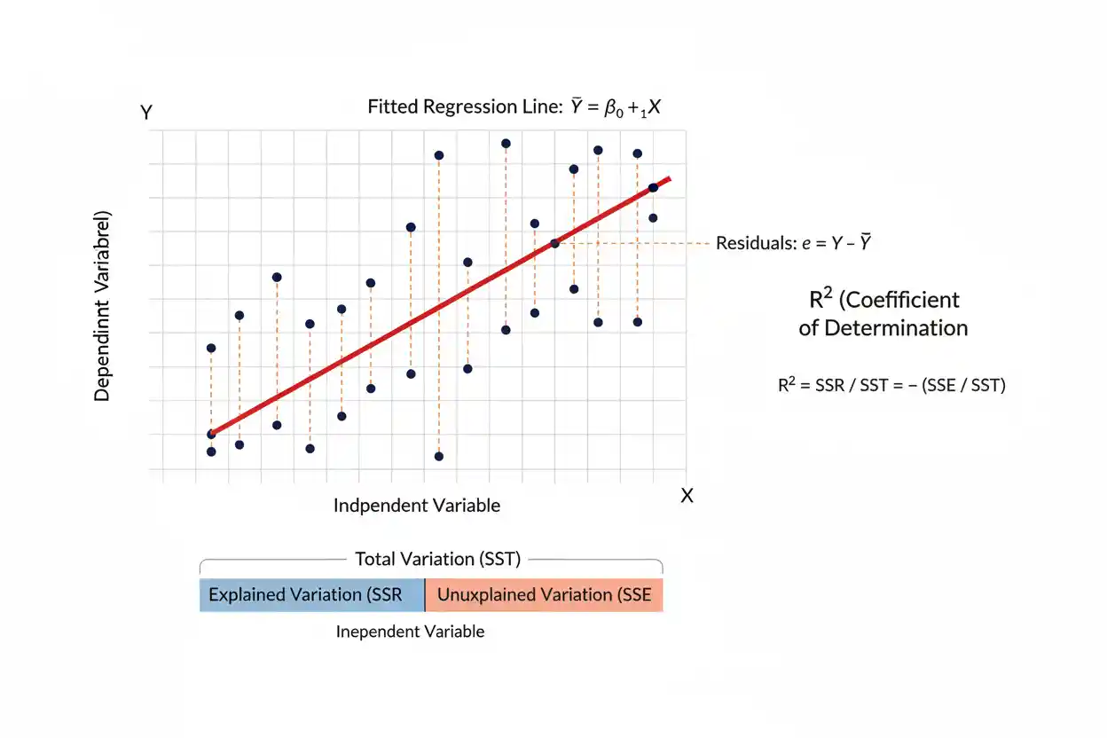
Coefficient Of Determination: Definition, Formula & Example

The coefficient of determination, usually written as R², is a statistical measure that describes how much of the variation in an outcome is accounted for by a fitted regression model relative to a baseline that predicts the outcome using its mean. It is one of the most widely reported measures of model fit because it converts the comparison between model error and total variation into a dimensionless quantity that is easy to interpret. In the standard ordinary least squares setting with an intercept, an R² of 0 means the model does no better than predicting the sample mean for every observation, while an R² of 1 means the fitted model reproduces every observed outcome exactly. Values between 0 and 1 describe intermediate levels of in-sample fit, although important exceptions arise when models omit an intercept or when R² is evaluated on new data.
The coefficient of determination does not tell whether the relationship is causal, whether the regression assumptions are satisfied, whether predictions are accurate enough for a practical decision, or whether every included variable is useful. It also should not be interpreted as the percentage of observations that the model predicts correctly. Its proper meaning concerns variation in the dependent variable and how much of that variation is represented by the fitted model under the relevant sum-of-squares decomposition. Understanding this distinction is essential for using R² correctly in regression analysis.
The coefficient of determination belongs to the broader field of Statistics & Probability and is especially relevant within Inference & Regression, where model fit, estimation, uncertainty, and interpretation must be considered together.
What Is the Coefficient of Determination?
The coefficient of determination measures the proportion of total observed variation in a response variable that is represented by a regression model relative to a mean-only baseline. It is normally denoted by:
R²
Suppose a dataset contains observed outcomes y₁, y₂, …, yₙ and fitted predictions ŷ₁, ŷ₂, …, ŷₙ. If the model predicts the observations closely, the unexplained residual variation will be small relative to the total variation in y, producing a larger R². If the fitted predictions offer little improvement over simply predicting the sample mean ȳ for every case, R² will be close to zero in the conventional least-squares-with-intercept setting.
The most commonly used formula is:
R² = 1 − SSE / SST
where SSE is the residual sum of squares and SST is the total sum of squares.
The residual sum of squares is:
SSE = Σ(yᵢ − ŷᵢ)²
The total sum of squares is:
SST = Σ(yᵢ − ȳ)²
Therefore:
R² = 1 − [Σ(yᵢ − ŷᵢ)² / Σ(yᵢ − ȳ)²]
This formula directly compares the prediction errors of the fitted regression model with the variability that would remain if every observation were predicted using only the sample mean.
What R² Measures
The coefficient of determination is fundamentally a relative measure of in-sample fit. The denominator SST represents the total squared variation of the observed response values around their mean. The numerator SSE represents the squared variation that remains unexplained after the fitted regression predictions are used.
If SSE is nearly as large as SST, the fitted model has removed little of the variation that was present relative to the mean-only baseline, so R² is close to zero. If SSE is much smaller than SST, the regression model fits the observed outcomes substantially better than that baseline, producing a larger R².
For example, suppose:
SST = 1,000
and:
SSE = 250
Then:
R² = 1 − 250/1,000
R² = 1 − 0.25
R² = 0.75
The model therefore accounts for 75% of the sample variation in the response relative to the mean-based benchmark used in the R² calculation. The remaining 25% is residual variation according to this decomposition.
This does not mean that 75% of individual outcomes are correctly predicted, that the predictors cause 75% of the outcome, or that the model is 75% accurate. Those are different claims.
Total, Explained, and Residual Variation
In an ordinary least squares regression containing an intercept, the total variation can be decomposed into explained and residual components.
The total sum of squares is:
SST = Σ(yᵢ − ȳ)²
The regression, or explained, sum of squares is:
SSR = Σ(ŷᵢ − ȳ)²
The residual sum of squares is:
SSE = Σ(yᵢ − ŷᵢ)²
For an ordinary least squares model fitted with an intercept:
SST = SSR + SSE
This makes it possible to express the coefficient of determination in two equivalent forms:
R² = SSR / SST
and:
R² = 1 − SSE / SST
The first form describes the proportion of total variation attributed to variation in the fitted values. The second describes R² as one minus the proportion of variation remaining in the residuals.
These identities depend on the standard least-squares decomposition. They should not be assumed to hold unchanged for every type of predictive model, loss function, or regression specification.
Worked Example
Suppose a simple regression analysis uses five observations with the following observed outcomes and fitted values:
| Observation | yᵢ | ŷᵢ |
|---|---|---|
| 1 | 2 | 2.2 |
| 2 | 3 | 3.1 |
| 3 | 5 | 4.0 |
| 4 | 4 | 4.9 |
| 5 | 6 | 5.8 |
The mean of the observed outcomes is:
ȳ = (2 + 3 + 5 + 4 + 6) / 5
ȳ = 4
First calculate the total sum of squares:
SST = Σ(yᵢ − ȳ)²
SST = (2 − 4)² + (3 − 4)² + (5 − 4)² + (4 − 4)² + (6 − 4)²
SST = 4 + 1 + 1 + 0 + 4
SST = 10
Now calculate the residual sum of squares:
SSE = Σ(yᵢ − ŷᵢ)²
SSE = (2 − 2.2)² + (3 − 3.1)² + (5 − 4.0)² + (4 − 4.9)² + (6 − 5.8)²
SSE = 0.04 + 0.01 + 1.00 + 0.81 + 0.04
SSE = 1.90
The coefficient of determination is therefore:
R² = 1 − 1.90/10
R² = 1 − 0.19
R² = 0.81
The model accounts for 81% of the observed variation in y relative to the sample-mean baseline. The remaining 19% appears in the residual sum of squares.
Because these fitted values come from an ordinary least squares line with an intercept, the explained sum of squares is:
SSR = SST − SSE
SSR = 10 − 1.90
SSR = 8.10
So the equivalent calculation is:
R² = 8.10 / 10
R² = 0.81
How to Interpret R²
An R² value is usually interpreted as a proportion of variation accounted for by the fitted model within the data used for the calculation.
If:
R² = 0.60
the model accounts for 60% of the total observed variation in the dependent variable relative to the mean-only baseline.
If:
R² = 0.95
the fitted model represents 95% of that variation.
If:
R² = 0.05
the model represents only 5% of the variation according to this measure.
The numerical interpretation is straightforward, but whether a particular value is good or bad is highly context-dependent. A value of 0.30 could be substantial in a field where outcomes are intrinsically noisy and affected by many unmeasured factors, while 0.90 could be inadequate in an engineering calibration task that requires extremely precise predictions.
There is no universal threshold at which an R² becomes acceptable.
R² Does Not Mean Prediction Accuracy
One of the most common mistakes is describing R² as a percentage accuracy score. The coefficient of determination is not classification accuracy, percentage error, or the fraction of predictions that are correct.
Suppose a model has:
R² = 0.80
This does not mean 80% of predictions are correct. Regression predictions for continuous outcomes are rarely exactly equal to observed values. R² instead means that the model accounts for 80% of the response variation relative to the mean-based benchmark under the applicable calculation.
Prediction quality should also be examined with measures directly tied to prediction error, such as residual magnitudes or an appropriate loss metric. A model can have a seemingly high R² while still making errors that are unacceptable for the intended application.
R² Does Not Establish Causation
A large coefficient of determination can occur when variables are strongly statistically associated, but association does not imply causation. A regression model may obtain a high R² because predictors are correlated with the outcome through confounding variables, common trends, indirect relationships, measurement artifacts, or purely predictive associations.
For example, two variables may both rise over time and therefore generate a strong fitted relationship even when neither causes the other. A high R² in such a model reflects statistical fit, not causal identification.
Causal conclusions require additional design and substantive assumptions, such as randomization, credible quasi-experimental structure, appropriate control of confounding, or a defensible causal model. R² alone provides none of these.
R² and Correlation
In simple ordinary least squares regression with one predictor and an intercept, the coefficient of determination has a special relationship with the Pearson correlation coefficient r between x and y:
R² = r²
If:
r = 0.80
then:
R² = 0.80²
R² = 0.64
In that specific setting, 64% of the variation in y is represented by the fitted linear relationship relative to the mean baseline.
However, the sign of the correlation disappears when it is squared. Both:
r = 0.80
and:
r = −0.80
produce:
R² = 0.64
R² therefore does not tell whether a simple linear relationship slopes upward or downward. The direction must be obtained from the regression coefficient or correlation itself.
The identity R² = r² should not be generalized mechanically to every multiple regression or nonlinear model. It is a special result for ordinary simple linear regression with an intercept.
Why R² Usually Falls Between 0 and 1
For an ordinary least squares regression fitted to the same data and containing an intercept, the model minimizes SSE and can always perform at least as well as the mean-only model. Therefore:
SSE ≤ SST
Substituting into:
R² = 1 − SSE/SST
gives the conventional range:
0 ≤ R² ≤ 1
An R² of 0 means that the fitted model provides no reduction in squared error compared with predicting ȳ for every observation. An R² of 1 means:
SSE = 0
so every fitted value equals its observed value.
This familiar 0-to-1 range depends on the standard in-sample ordinary least squares setup with an intercept. Outside that setting, negative R² values can occur.
Can R² Be Negative?
Yes. A coefficient of determination can be negative under some definitions and evaluation settings.
Suppose R² is calculated as:
R² = 1 − SSE/SST
and the model produces:
SSE > SST
Then:
SSE/SST > 1
which implies:
R² < 0
A negative value means the model’s squared prediction error is worse than the relevant mean-based baseline.
This commonly occurs when R² is evaluated on new test data, because the fitted model is no longer guaranteed to outperform the test-set mean benchmark. Negative values can also arise with regression specifications that omit an intercept, depending on how the sum of squares is defined.
Therefore, the claim that R² must always lie between 0 and 1 is only correct under the conventional in-sample least-squares conditions.
R² With and Without an Intercept
The standard interpretation of R² relies heavily on a model containing an intercept. With an intercept, ordinary least squares residuals have properties that produce the familiar sum-of-squares decomposition:
SST = SSR + SSE
Without an intercept, those identities may not hold in the same way. Software can also use different definitions of R² for no-intercept models, which can produce values that behave differently from the conventional measure.
A regression forced through the origin should therefore not have its R² interpreted automatically as though it were directly comparable with an ordinary intercept model.
The intercept decision should be based on the structure of the problem, not on a desire to manipulate the reported fit statistic.
Sample R² vs Population Relationships
The R² reported from a fitted sample is a statistic calculated from observed data. It should not automatically be treated as an exact population quantity.
A different random sample from the same population will generally produce different regression coefficients, predictions, residuals, and R² values. The sample coefficient of determination therefore contains sampling variability.
This distinction is especially important with small datasets, where an apparently strong in-sample fit may be unstable. Statistical inference and model validation are needed when the objective is to make broader conclusions beyond the observed sample.
The central limit theorem provides important foundations for many sampling-distribution arguments in statistics, but it does not make a particular observed R² automatically reliable or normally distributed. Inference for regression fit requires results specific to the model and statistic being studied.
Adding Predictors and R²
In ordinary least squares regression fitted to the same observations, adding another predictor cannot decrease the conventional training R². The existing model is still available as a special case in which the new coefficient is effectively zero, so the expanded model can obtain an SSE that is equal to or smaller than before.
Therefore:
R²new ≥ R²old
for nested ordinary least squares models evaluated on the same training data under the conventional setup.
This property can be useful, but it also creates a limitation. Adding irrelevant predictors can slightly increase R² even when they provide little genuine explanatory or predictive value. A larger raw R² therefore does not automatically mean a better model.
Model comparison should consider the research objective, parameter complexity, validation performance, assumptions, and uncertainty rather than maximizing R² mechanically.
R² and Overfitting
Overfitting occurs when a model captures sample-specific noise rather than a stable underlying pattern. Because training R² tends to increase as flexibility is added, an overfit model can display an impressive coefficient of determination in the data used to estimate it.
Its performance can deteriorate sharply on new observations.
Imagine a dataset with 50 observations and a highly flexible model containing many predictors. It may achieve:
R² = 0.98
in the training sample, yet make poor predictions on future data. The large training R² describes fit to the observed sample rather than guaranteed generalization.
This is why predictive modeling usually separates model fitting from model evaluation. Out-of-sample error, cross-validation, and other validation procedures address questions that the training R² alone cannot answer.
Adjusted R²
Adjusted R² modifies the ordinary coefficient of determination to account for the number of predictors relative to the sample size. A common formula for a regression with n observations and k explanatory variables is:
Adjusted R² = 1 − [(1 − R²)(n − 1) / (n − k − 1)]
Unlike ordinary R², adjusted R² can decrease when a new predictor fails to improve the model enough to compensate for the added complexity.
Suppose:
R² = 0.80
n = 100
k = 4
Then:
Adjusted R² = 1 − [(1 − 0.80)(99) / 95]
Adjusted R² = 1 − (19.8 / 95)
Adjusted R² ≈ 0.792
The adjusted value is slightly smaller because it incorporates a complexity penalty.
Adjusted R² can be useful when comparing related linear regression models with different numbers of predictors, but it is not a universal model-selection criterion and does not replace validation or substantive judgment.
R² vs Adjusted R²
Ordinary R² answers how much variation the fitted model accounts for relative to the baseline. Adjusted R² modifies that value based on model complexity.
For ordinary R²:
adding predictors cannot reduce training R²
For adjusted R²:
adding a weak predictor can reduce the statistic
This makes adjusted R² less mechanically favorable toward larger models. However, both quantities are still based on in-sample fit and should not be interpreted as direct measures of future predictive accuracy.
A model should not be selected solely because it has the highest adjusted R² when other issues such as residual structure, instability, data leakage, scientific plausibility, or poor external validation are present.
Coefficient of Determination vs Effect Size
The coefficient of determination can communicate the magnitude of model fit, but it should not be confused with every other type of effect size. Different statistical questions require different measures.
For example, Cohen D measures a standardized difference between means in common two-group settings. R² instead describes variation accounted for by a regression model relative to a baseline.
An R² of 0.40 and a Cohen d of 0.40 therefore do not have the same interpretation. They arise from different mathematical structures and describe different features of data.
Selecting an effect-size measure should follow the research question and model rather than the desire to report a familiar number.
R² and Statistical Significance
A regression model can have a low R² while containing a statistically significant predictor, particularly when the sample is large. Conversely, a model can show a seemingly substantial R² in a small sample while its parameter estimates remain uncertain.
R² and statistical significance answer different questions.
R² asks how much observed variation is accounted for by the fitted model relative to a specified baseline. A significance test asks whether the sample provides evidence against a particular null hypothesis.
A model-fit statistic should therefore not be used as a replacement for hypothesis testing. Likewise, a small p-value does not imply a large R² or practical importance.
The concepts of critical value and hypothesis-testing reference distributions belong to the inferential decision framework, whereas R² primarily summarizes fit.
R² in Multiple Regression
In multiple regression, the outcome is modeled using several predictors simultaneously. The coefficient of determination continues to compare the residual variation from the fitted model with total variation around the outcome mean.
The usual formula remains:
R² = 1 − SSE/SST
Suppose a model predicting annual sales from price, advertising expenditure, store size, and market characteristics produces:
SST = 50,000
SSE = 15,000
Then:
R² = 1 − 15,000/50,000
R² = 1 − 0.30
R² = 0.70
The fitted model accounts for 70% of the observed variation in annual sales relative to the mean-only baseline.
That result does not mean each predictor accounts for 17.5%. Predictor contributions generally overlap and depend on correlations among explanatory variables. The overall R² cannot ordinarily be divided equally among predictors.
R² Does Not Identify Important Predictors
A high overall coefficient of determination says nothing by itself about which predictor is responsible for the fit. In multiple regression, several variables can carry overlapping information, and the estimated contribution of one predictor can depend on which other variables are included.
For example, two predictors may be strongly correlated with one another and jointly produce a high R². Removing either one individually might have only a limited effect because the other contains similar information.
Determining predictor importance requires additional analysis, such as regression coefficients, partial comparisons, model-based contribution measures, or domain-specific interpretation. R² is an overall model-fit statistic rather than a variable-importance ranking.
R² and Residual Analysis
A high R² does not guarantee that a regression model is well specified. Residuals may still display curvature, changing variance, dependence, extreme outliers, or other patterns inconsistent with the fitted model.
Consider a nonlinear relationship fitted with a straight line. If the overall trend is strong, R² could be high even though the residual plot reveals systematic curvature. The statistic summarizes the amount of squared variation represented by the model but does not reveal the shape of the remaining errors.
Residual diagnostics therefore provide information that R² cannot.
Model evaluation should ask both how much variation is represented and whether the remaining structure is consistent with the assumptions and intended use of the model.
High R² Can Be Misleading
A large coefficient of determination can look persuasive while concealing important problems. Time-series variables that trend together can generate high R² values without a meaningful structural relationship. Outliers can strongly influence both fitted regression coefficients and sums of squares. Data leakage can produce excellent fit by allowing the model to use information that would not actually be available when predictions are made.
A high R² can also coexist with severe extrapolation risk. A model may fit extremely well within the observed x-range but make unreliable predictions far outside that range.
The statistic should therefore be interpreted as one component of model assessment rather than as a final verdict on model quality.
Low R² Does Not Automatically Mean a Bad Model
A low R² can be entirely reasonable when the outcome contains substantial natural variability or when the objective is estimating a specific association rather than predicting individual outcomes.
Suppose a treatment variable explains only a small fraction of variation in a health outcome because genetics, environment, measurement noise, and numerous other influences contribute to the response. The treatment effect could still be scientifically important even if the overall R² is modest.
Similarly, models of human behavior often encounter far more unexplained variation than models of tightly controlled physical systems.
Whether R² is satisfactory depends on what the model is intended to accomplish.
Coefficient of Determination vs Chi-Square Statistics
The coefficient of determination should not be confused with chi-square test statistics. A chi-square test of independence evaluates whether two categorical variables are associated by comparing observed and expected cell counts. A chi-square goodness of fit test compares an observed categorical distribution with a specified expected distribution.
R² is instead primarily associated with regression fit for quantitative outcomes under its conventional definition.
A chi-square value of 20 does not mean 20% of variation is explained, and an R² of 0.60 does not represent a chi-square significance level. The measures answer fundamentally different questions.
R² and Model Comparison
R² can help compare certain regression models when they use the same response variable and are fitted to the same observations. If one model produces:
R² = 0.65
and another produces:
R² = 0.78
the second model achieves a greater reduction in residual squared variation relative to the common baseline.
However, this comparison does not by itself establish that the second model is preferable. If it contains many additional predictors, the improvement could represent overfitting. If the models use different outcome transformations, samples, weighting schemes, or definitions of total variation, direct comparison can become misleading.
Model comparison requires consistent data and definitions as well as consideration of complexity and generalization.
Out-of-Sample R²
The coefficient of determination can also be calculated on test or validation data to compare prediction errors with a baseline.
A common form is:
R²test = 1 − SSEtest/SSTtest
where:
SSEtest = Σ(yᵢ − ŷᵢ)²
and SSTtest measures variation around the relevant test-set baseline.
Unlike ordinary training R² from least squares with an intercept, out-of-sample R² can easily be negative. If the model predicts new observations worse than the baseline mean, then:
SSEtest > SSTtest
and therefore:
R²test < 0
A negative out-of-sample value can be extremely informative because it reveals that impressive training fit has not translated into useful predictive performance.
What Is a Good R²?
There is no universal good R². Appropriate values depend on the field, outcome variability, model purpose, measurement precision, sample quality, and consequences of prediction error.
A predictive system controlling a manufacturing process may require R² extremely close to 1 because small unexplained deviations are costly. A social-science model may produce useful insight with a much lower value because individual behavior contains large amounts of irreducible variation.
The correct question is not simply “Is R² high?” It is whether the model fit is adequate for the decision, prediction, or scientific question being addressed.
Comparisons with realistic benchmarks and competing models are usually more informative than universal thresholds.
Common Misconceptions
A frequent misconception is that R² measures the percentage of predictions that are correct. It does not. It measures variation accounted for relative to a baseline.
Another error is interpreting an R² of 0.70 as evidence that x causes 70% of y. R² is not a causal proportion.
It is also incorrect to assume that the model with the highest training R² is automatically best. Additional predictors and flexibility can increase training fit while reducing generalization.
Another misconception is that R² must always lie between 0 and 1. That range applies in the standard in-sample ordinary least squares model with an intercept, but negative values can arise in other settings.
Finally, a high R² does not guarantee that assumptions are satisfied, residuals behave properly, coefficients are stable, or the model is suitable for extrapolation.
How to Calculate the Coefficient of Determination
Begin by calculating the mean of the observed response values:
ȳ = Σyᵢ / n
Next calculate the total sum of squares:
SST = Σ(yᵢ − ȳ)²
Then obtain the model predictions ŷᵢ and calculate the residual sum of squares:
SSE = Σ(yᵢ − ŷᵢ)²
Finally calculate:
R² = 1 − SSE/SST
In an ordinary least squares regression with an intercept, the explained sum of squares can also be calculated:
SSR = Σ(ŷᵢ − ȳ)²
and:
R² = SSR/SST
Before interpreting the result, verify that the definition being used matches the regression specification and evaluation setting.
Frequently Asked Questions
What is the coefficient of determination?
The coefficient of determination, R², measures how much of the observed variation in a response variable is accounted for by a fitted regression model relative to a mean-based baseline.
What is the formula for R²?
The most common formula is:
R² = 1 − SSE/SST
where SSE is the residual sum of squares and SST is the total sum of squares.
What does R² = 0.80 mean?
Under the conventional interpretation, the fitted model accounts for 80% of the observed variation in the response relative to the mean-only baseline. It does not mean that 80% of predictions are correct.
What does R² = 0 mean?
In an ordinary least squares model with an intercept, R² = 0 means the model provides no improvement in squared-error fit over predicting the sample mean for every observation.
What does R² = 1 mean?
R² = 1 means the model fits the observed response values perfectly in the sample:
SSE = 0
Every residual is therefore zero.
Can R² be negative?
Yes. Negative R² can occur when the model performs worse than the baseline used in the calculation, especially on out-of-sample data or in some models without an intercept.
Is a higher R² always better?
Not necessarily. A higher training R² means better in-sample squared-error fit relative to the same baseline, but it can result from unnecessary predictors or overfitting. Model quality requires broader evaluation.
Does a high R² prove causation?
No. R² measures statistical fit, not causal identification.
Is R² the same as correlation?
No. In simple linear regression with one predictor and an intercept, R² equals the squared Pearson correlation between x and y. That special relationship does not make the two measures generally identical.
Can R² decrease when a predictor is added?
Ordinary training R² cannot decrease when another predictor is added to a nested ordinary least squares model fitted to the same observations. Adjusted R², however, can decrease.
What is adjusted R²?
Adjusted R² modifies ordinary R² to account for the number of predictors relative to the sample size. It penalizes model expansion that provides too little additional fit.
Does a low R² mean the model is useless?
No. A low R² may still accompany an important and precisely estimated relationship, particularly in fields where outcomes contain substantial natural variability.
Does a high R² guarantee accurate future predictions?
No. High in-sample R² can coexist with poor out-of-sample performance, particularly when the model overfits or the future data differ from the training sample.
What is the difference between R² and a chi-square statistic?
R² summarizes regression fit relative to variation in a quantitative outcome. Chi-square statistics typically compare observed and expected categorical frequencies. They measure different statistical properties.
Should R² be reported by itself?
Usually not. Interpretation is stronger when R² is considered alongside the regression coefficients, residual behavior, uncertainty, sample size, validation results, and the practical purpose of the model.
Key Takeaway
The coefficient of determination is a regression fit measure that compares residual variation with the total variation in an outcome. Its most common formula is:
R² = 1 − SSE/SST
with:
SSE = Σ(yᵢ − ŷᵢ)²
and:
SST = Σ(yᵢ − ȳ)²
For an ordinary least squares model with an intercept, the equivalent explained-variation form is:
R² = SSR/SST
An R² near 1 indicates that the fitted model represents a large share of the observed variation relative to the mean baseline, while an R² near 0 indicates little improvement over that baseline. The statistic does not measure percentage accuracy, establish causation, identify important predictors, guarantee valid assumptions, or prove that a model will perform well on new data. Its value is greatest when it is interpreted as one precise component of model evaluation rather than as a complete measure of model quality.



