
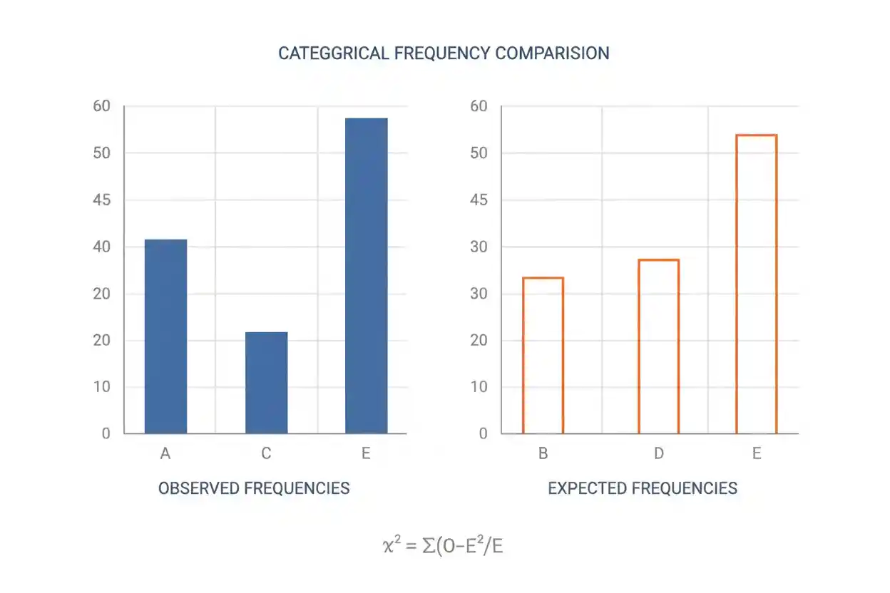
Chi-Square Goodness Of Fit: Definition, Formula & Example

The chi-square goodness of fit test is an inferential statistical procedure used to determine whether observed counts across categories are consistent with a specified probability distribution. It is appropriate when one categorical variable produces frequencies such as counts of customers choosing different options, outcomes from repeated dice rolls, product defects by type, or responses distributed across survey categories. The test compares the counts actually observed with the counts that would be expected if a stated null hypothesis were correct. Differences between observed and expected counts are converted into a chi-square test statistic, with larger discrepancies producing larger values of the statistic. The result can then be evaluated against a chi-square reference distribution to calculate a p-value or compare the statistic with a critical value.
Importantly, the procedure tests an entire categorical distribution rather than estimating whether one particular category alone differs from expectation. It also does not measure the practical importance of a discrepancy simply because a result is statistically significant. Correct use requires independent observations, mutually exclusive categories, appropriately specified expected probabilities, and expected frequencies large enough for the usual chi-square approximation to be reliable.
The test sits within the broader field of Statistics & Probability and is one of several procedures covered by Inference & Regression. Its specific purpose is narrow: testing whether one observed categorical frequency distribution fits a hypothesized distribution.
What Is the Chi-Square Goodness of Fit Test?
A chi-square goodness of fit test compares observed frequencies with expected frequencies for a single categorical variable. Suppose a population is divided into k mutually exclusive categories. Under the null hypothesis, each category has a specified probability. If a sample of n observations is collected, those probabilities imply expected counts for the categories. The test asks whether the differences between the observed and expected counts are small enough to be reasonably explained by random sampling variation or large enough to provide evidence against the hypothesized distribution.
If Oᵢ is the observed frequency for category i and Eᵢ is its expected frequency, the Pearson chi-square goodness of fit statistic is:
χ² = Σ[(Oᵢ − Eᵢ)² / Eᵢ]
The summation is taken across all k categories. Every category contributes a nonnegative quantity because the observed-minus-expected difference is squared. A category contributes more to χ² when its observed frequency differs substantially from expectation relative to the size of its expected count.
A value of χ² near zero indicates that observed counts are close to expected counts. A larger value indicates greater disagreement. Whether a particular value is sufficiently large to reject the null hypothesis depends on the degrees of freedom and the chosen significance level.
Observed Frequencies and Expected Frequencies
Observed frequencies are simply the category counts found in the data. If 120 rolls of a die produce 10 ones, 14 twos, 18 threes, 22 fours, 26 fives, and 30 sixes, those six numbers are the observed frequencies.
Expected frequencies are the counts predicted under the null hypothesis. If the null hypothesis states that the die is fair, every face has probability 1/6. With n = 120 rolls, the expected count for each outcome is therefore 20.
In general, if category i has hypothesized probability pᵢ, its expected frequency is:
Eᵢ = npᵢ
The expected frequencies should sum to the total sample size:
ΣEᵢ = n
Similarly, the hypothesized category probabilities must sum to 1:
Σpᵢ = 1
This distinction between probability and count is important. A probability such as 0.25 is not inserted directly into the denominator of the chi-square statistic when the observed values are counts. It must first be converted to the corresponding expected frequency by multiplying by n.
Null and Alternative Hypotheses
The null hypothesis specifies the categorical distribution being tested. If the hypothesized category probabilities are p₁₀, p₂₀, …, pₖ₀, the null can be represented as:
H₀: p₁ = p₁₀, p₂ = p₂₀, …, pₖ = pₖ₀
For a fair six-sided die:
H₀: p₁ = p₂ = p₃ = p₄ = p₅ = p₆ = 1/6
The alternative hypothesis is that the complete specified distribution does not hold. In practical terms:
H₁: at least one true category probability differs from its value specified under H₀
This does not mean the test initially identifies which category is different. A significant overall result says that the observed distribution provides evidence against the complete null distribution. Determining where the important discrepancies occur requires examination of category contributions or an appropriate follow-up analysis.
Chi-Square Goodness of Fit Formula
The test statistic is:
χ² = Σ[(Oᵢ − Eᵢ)² / Eᵢ]
where Oᵢ is the observed frequency in category i and Eᵢ is the expected frequency under the null hypothesis.
The statistic has three important features. First, subtracting Eᵢ from Oᵢ measures the discrepancy between observation and expectation. Second, squaring the difference prevents positive and negative discrepancies from canceling one another. Third, dividing by Eᵢ scales each squared discrepancy relative to the expected size of its category.
The contribution from a single category is therefore:
χ²ᵢ = (Oᵢ − Eᵢ)² / Eᵢ
and the total statistic is the sum of the individual contributions:
χ² = χ²₁ + χ²₂ + … + χ²ₖ
Because every contribution is nonnegative:
χ² ≥ 0
A statistic of exactly zero occurs only when every observed count equals its corresponding expected count.
Worked Example: Testing Whether a Die Is Fair
Suppose a six-sided die is rolled 120 times. The observed frequencies are:
| Die Face | Observed Oᵢ | Expected Eᵢ |
|---|---|---|
| 1 | 10 | 20 |
| 2 | 14 | 20 |
| 3 | 18 | 20 |
| 4 | 22 | 20 |
| 5 | 26 | 20 |
| 6 | 30 | 20 |
If the die is fair, every outcome has probability 1/6. Since n = 120:
Eᵢ = 120 × (1/6) = 20
The chi-square contribution for face 1 is:
(10 − 20)² / 20 = 100 / 20 = 5
For face 2:
(14 − 20)² / 20 = 36 / 20 = 1.8
For face 3:
(18 − 20)² / 20 = 4 / 20 = 0.2
Also, For face 4:
(22 − 20)² / 20 = 4 / 20 = 0.2
For face 5:
(26 − 20)² / 20 = 36 / 20 = 1.8
For face 6:
(30 − 20)² / 20 = 100 / 20 = 5
Adding the contributions gives:
χ² = 5 + 1.8 + 0.2 + 0.2 + 1.8 + 5
χ² = 14
Because the null hypothesis completely specifies six category probabilities and no parameters were estimated from these same data, the degrees of freedom are:
df = k − 1
df = 6 − 1 = 5
For χ² = 14 with df = 5, the upper-tail p-value is approximately:
p ≈ 0.0156
If the analysis uses α = 0.05, then:
p < α
The null hypothesis is therefore rejected at the 5% significance level. The data provide statistical evidence that the distribution of die outcomes differs from the equal-probability distribution expected from a fair die.
That conclusion should be stated carefully. The test does not establish why the distribution differs, nor does it prove a specific physical defect in the die. It identifies evidence of disagreement between the observed frequencies and the hypothesized distribution.
Degrees of Freedom
For a goodness of fit test with k categories and fully specified category probabilities, the usual degrees of freedom are:
df = k − 1
One degree of freedom is lost because the category counts must add to the fixed total n. Once the counts of k − 1 categories are known, the final category count is determined by the total.
For example, if four categories contain 100 observations in total and the first three observed counts are 20, 30, and 25, the fourth count must be:
100 − 20 − 30 − 25 = 25
It is therefore not freely variable.
When one or more parameters of the hypothesized distribution are estimated from the same sample before expected frequencies are calculated, additional degrees of freedom may be lost. A common form is:
df = k − 1 − m
where m is the number of independently estimated parameters used to determine the expected probabilities. This adjustment is model-dependent, so k − 1 should not be applied mechanically when expected probabilities were fitted from the data.
Why the Chi-Square Distribution Is Used
Under H₀ and suitable regularity conditions, the Pearson goodness of fit statistic has an approximate chi-square sampling distribution. The approximation becomes useful because random differences between observed and expected counts can then be evaluated against a known reference distribution.
The chi-square distribution is nonnegative and generally right-skewed, particularly at low degrees of freedom. Its precise shape changes with df. As degrees of freedom increase, its center shifts rightward and its relative skewness decreases.
The test is therefore an upper-tail procedure. Very large χ² values indicate more disagreement with H₀ than would normally be expected from sampling variability alone. Small values are not evidence against H₀.
This use of an asymptotic reference distribution has conceptual connections with the central limit theorem, since large-sample approximations frequently emerge from the behavior of standardized random quantities. However, the chi-square goodness of fit procedure has its own test statistic, assumptions, degrees of freedom, and reference distribution.
Calculating the P-Value
Once χ² and df have been determined, the p-value is the probability, assuming H₀ and the statistical model are correct, of obtaining a chi-square statistic at least as large as the statistic actually observed:
p-value = P(Χ²df ≥ χ²observed | H₀)
A small p-value indicates that the observed discrepancies would be relatively unusual under the null distribution. If the p-value is below the prespecified significance level α, the usual decision is to reject H₀.
A p-value is not the probability that H₀ is true. For example, p = 0.02 does not mean there is a 2% probability that the hypothesized distribution is correct. It describes the tail behavior of the test statistic under the assumption that H₀ is true.
Using a Critical Value Instead
A goodness of fit test can also be performed using a critical value instead of calculating the exact p-value. The critical value depends on the selected α and the degrees of freedom.
The decision rule has the form:
Reject H₀ if χ²observed > χ²critical
For the die example, df = 5. At α = 0.05, the relevant upper-tail chi-square critical value is approximately 11.07. Because:
14 > 11.07
the null hypothesis is rejected.
The p-value and critical-value approaches lead to the same decision when the same significance level and reference distribution are used. They are two ways of evaluating the same test statistic.
Conditions for a Chi-Square Goodness of Fit Test
The first requirement is that the response variable be categorical and represented by counts. The observations must be assigned to mutually exclusive categories so that one observation does not contribute simultaneously to multiple categories in the same goodness of fit calculation. The test is not designed for comparing means of quantitative measurements.
Independence is also important. One observation should not automatically determine or strongly duplicate another observation under the sampling design. Repeated measurements on the same individual, clustered observations, matched data, or other forms of dependence can invalidate the ordinary reference distribution if handled as though every count came from an independent observation.
The expected counts must also be sufficiently large for the chi-square approximation to work adequately. A frequently taught guideline is that expected counts should generally be at least 5, but this is a practical approximation guideline rather than a universal mathematical boundary. The quality of the approximation depends on the structure of the problem, and very sparse categories may require combining scientifically defensible categories or using a more appropriate exact or simulation-based method.
Finally, the hypothesized probabilities must be specified correctly. If they are estimated from the sample, the degrees of freedom and sometimes the entire testing procedure may need adjustment.
Expected Counts Must Come From H₀
Expected frequencies should never be chosen merely because they make the observed data appear close to expectation. They must follow logically from the null hypothesis.
Suppose a manufacturer historically expects four defect categories in proportions 0.40, 0.30, 0.20, and 0.10. In a sample of 500 defects, the expected counts are:
E₁ = 500 × 0.40 = 200
E₂ = 500 × 0.30 = 150
E₃ = 500 × 0.20 = 100
E₄ = 500 × 0.10 = 50
The expected distribution is therefore 200, 150, 100, and 50—not four equal counts of 125. Equal expected frequencies are appropriate only when H₀ actually specifies equal category probabilities.
Worked Example With Unequal Expected Probabilities
Suppose an organization expects customer inquiries to arrive through three channels in proportions 50%, 30%, and 20%. A sample of n = 200 inquiries produces observed counts of 110, 52, and 38.
The expected frequencies are:
E₁ = 200 × 0.50 = 100
E₂ = 200 × 0.30 = 60
E₃ = 200 × 0.20 = 40
The chi-square statistic is:
χ² = (110 − 100)² / 100 + (52 − 60)² / 60 + (38 − 40)² / 40
χ² = 100/100 + 64/60 + 4/40
χ² ≈ 1 + 1.067 + 0.100
χ² ≈ 2.167
With three fully specified categories:
df = 3 − 1 = 2
The discrepancies are relatively modest compared with the expected counts. The resulting chi-square statistic therefore provides much less evidence against H₀ than the die example. This illustrates why absolute differences alone are insufficient: the test evaluates each difference relative to the corresponding expected frequency.
Which Categories Contribute Most?
When the overall test is significant, examining the individual chi-square contributions can show which categories are responsible for much of the discrepancy:
contributionᵢ = (Oᵢ − Eᵢ)² / Eᵢ
In the die example, categories 1 and 6 each contributed 5 to the total χ² of 14, substantially more than the middle outcomes. That indicates where the strongest departures from the null model occur.
However, contribution size does not itself provide the full inferential framework for making multiple category-specific claims. If an analysis proceeds to formal follow-up comparisons, issues such as multiple testing and the specific research question must be considered. The overall goodness of fit test should therefore remain distinct from a collection of separate unadjusted tests.
Chi-Square Goodness of Fit vs Chi-Square Test of Independence
The goodness of fit test and the chi-square test of independence use related mathematics but answer different questions.
A goodness of fit test studies one categorical variable. It asks whether that variable follows a specified distribution. For example, it might ask whether six die outcomes occur with equal probabilities or whether customer preferences follow a predefined 40%-35%-25% allocation.
A test of independence studies two categorical variables arranged in a contingency table. It asks whether the variables are statistically associated. For example, it might test whether product preference is associated with customer region.
The difference is conceptual as well as computational. Goodness of fit compares one observed distribution with a specified distribution, whereas independence compares the joint pattern of two categorical variables with the pattern expected under statistical independence.
Chi-Square Goodness of Fit vs a Test of a Mean
The goodness of fit statistic is based on categorical frequency counts. It is not a replacement for procedures designed to test population means.
If the research question concerns whether a population mean equals a specified value, a one-sample t-test or a suitable z-based procedure may be relevant depending on the assumptions and available information. Transforming quantitative observations into arbitrary categories simply to use a chi-square goodness of fit test can discard information unnecessarily.
The statistical procedure should follow the measurement scale and the research question, not the other way around.
Goodness of Fit and Sampling Distributions
Like other inferential procedures, the test depends on the concept of a sampling distribution. Imagine repeating the same study many times while H₀ is true, calculating the Pearson χ² statistic for every sample. Under the required conditions and as the approximation becomes appropriate, the distribution of those statistics is described by the relevant chi-square reference distribution.
This repeated-sampling interpretation explains the logic of the p-value. The p-value identifies how far into the upper tail the observed statistic lies under the null model; it does not compare the observed counts with a subjective notion of what “looks close enough.”
Statistical Significance Is Not Effect Size
A chi-square goodness of fit statistic can become statistically significant when a very large sample detects comparatively small departures from the hypothesized proportions. Consequently, rejecting H₀ does not automatically mean the discrepancy is substantively important.
Statistical significance addresses whether the data provide evidence against a specified null distribution. Effect size addresses the magnitude of a difference or relationship. Those are distinct questions.
Similarly, Cohen D is a standardized effect-size measure typically associated with differences between quantitative means, not the goodness of fit statistic for categorical frequencies. A significant χ² result should not be translated into Cohen’s d without a valid reason and an appropriate model.
The key principle is simple: statistical evidence and practical importance must be interpreted separately.
Chi-Square Goodness of Fit Is Not R²
The goodness of fit terminology can also cause confusion with model-fit measures used elsewhere in statistics. The coefficient of determination, commonly written R², describes a proportion of variation associated with a regression model under its usual definition. It is not the same quantity as a Pearson chi-square goodness of fit statistic.
A χ² value of 12 therefore does not mean that a model explains 12% of the variation, nor does a larger χ² indicate better fit in this test. For the Pearson goodness of fit test described here, larger χ² values indicate greater discrepancy between observed and expected frequencies.
Effect of Sample Size
Sample size affects both the reliability of the chi-square approximation and the sensitivity of the test. Small samples can produce sparse expected frequencies, weakening the approximation to the reference distribution. Very large samples, in contrast, can make the test sensitive to relatively small proportional discrepancies.
Consider a category expected to contain half of all observations. A deviation of 2 percentage points may be difficult to distinguish from sampling noise in a small sample but highly statistically detectable in a sample containing hundreds of thousands of observations. The substantive importance of that difference does not automatically increase merely because the p-value becomes smaller.
This is why a complete interpretation should consider the actual observed and expected proportions, sample size, context, and an appropriate measure of discrepancy rather than reporting only “significant” or “not significant.”
What Happens When Expected Counts Are Small?
The chi-square reference distribution is an approximation. When expected counts are very small, the discrete distribution of the observed frequencies may not be represented adequately by that approximation.
A common classroom guideline recommends expected counts of approximately 5 or greater, but the appropriate response to sparse data depends on the problem. Categories should not be combined merely to force compliance with a numerical rule if the combination destroys an important scientific distinction. Conversely, categories that are naturally compatible may sometimes be combined before analysis if doing so is substantively justified.
For some small-sample categorical problems, exact procedures or simulation methods may be more suitable. The essential point is that a large-sample approximation should not be treated as exact when the expected frequency structure provides little support for it.
Independence and Sampling Design
A large total sample does not compensate for a flawed dependence structure. Suppose 1,000 responses are collected, but they come from only 100 households with 10 nearly identical responses per household. Treating all 1,000 responses as independent can exaggerate the effective information in the sample.
The ordinary goodness of fit statistic assumes a sampling mechanism under which the categorical counts have the appropriate multinomial-type variability under H₀. Complex survey designs, repeated observations, clusters, or temporal dependence can alter that variability. In such cases, a specialized method that accounts for the design may be necessary.
Understanding how observations were generated is therefore as important as calculating χ² correctly.
Type I and Type II Errors
Rejecting H₀ is a decision made under uncertainty. A Type I error occurs when H₀ is rejected even though the specified null distribution is actually correct. The significance level α controls the long-run probability of this error under the test’s assumptions.
A Type II error occurs when the test fails to reject H₀ even though the actual population distribution differs from the null specification. The probability of detecting a particular departure when it truly exists is related to statistical power.
These concepts make clear why “fail to reject H₀” should not be rewritten as “prove H₀ is true.” A nonsignificant result may reflect a distribution genuinely close to H₀, insufficient sample information, small departures, or other limitations of the design.
Interpreting a Significant Result
Suppose a test produces:
χ² = 14.0
df = 5
p ≈ 0.0156
At α = 0.05, a suitable interpretation is that the observed categorical distribution provides statistically significant evidence against the distribution specified by H₀.
An unsuitable interpretation would be that there is a 1.56% chance H₀ is true. Another unsuitable statement would be that the alternative distribution has been proved. The test provides evidence about compatibility between the observed data and the null model under specified assumptions; it does not assign a posterior probability to H₀.
After a significant result, the observed proportions and individual category discrepancies should be examined to understand the practical pattern.
Interpreting a Nonsignificant Result
Suppose another test gives:
χ² = 2.17
df = 2
p > 0.05
The appropriate decision at α = 0.05 is to fail to reject H₀. That means the sample does not provide sufficiently strong evidence, using this test and significance threshold, that the population distribution differs from the hypothesized distribution.
It does not establish that the hypothesized probabilities are exactly correct. Statistical tests are designed to evaluate evidence against a null model, not to certify exact equality from a finite sample.
Common Mistakes
One common error is using percentages as Oᵢ and counts as Eᵢ. Both quantities in the Pearson formula must be represented on the same frequency scale. If observed data are counts, expected values must also be counts.
Another mistake is assuming equal expected frequencies without a null hypothesis that actually predicts equal probabilities. The correct expected values come from H₀, whether the probabilities are equal or unequal.
A third mistake is using df = k − 1 when parameters were estimated from the same data and the model requires a degrees-of-freedom adjustment. Degrees of freedom follow the structure of the null model.
Researchers can also misinterpret a large χ² statistic as evidence of “better fit.” In this test, the opposite is true: larger values represent larger standardized discrepancies from the expected distribution.
Finally, statistical significance should not be confused with practical importance. A very large dataset can expose minor departures that have little operational consequence, while a smaller study can lack power to detect a meaningful difference.
A Practical Chi-Square Goodness of Fit Workflow
Begin by defining the categorical variable and the hypothesized probabilities before interpreting the observed deviations. Make sure the categories are mutually exclusive and collectively represent the outcomes relevant to the model. State H₀ as the complete proposed distribution and H₁ as a departure from that distribution.
Next, convert each hypothesized probability to an expected count using Eᵢ = npᵢ. Verify that the expected counts add to n and assess whether they are sufficiently large for a chi-square approximation. Then calculate each category contribution, sum those values to obtain χ², and determine the correct degrees of freedom.
Finally, evaluate the result using a p-value or critical value and report the conclusion in terms of the original categorical distribution. If H₀ is rejected, inspect the category discrepancies to understand where the disagreement lies, while keeping the distinction between statistical significance and substantive importance clear.
Frequently Asked Questions
What does a chi-square goodness of fit test measure?
It measures how strongly an observed set of categorical frequencies disagrees with frequencies expected under a specified probability distribution. The Pearson statistic aggregates squared observed-minus-expected discrepancies after scaling each one by its expected frequency.
What is the chi-square goodness of fit formula?
The standard Pearson statistic is:
χ² = Σ[(Oᵢ − Eᵢ)² / Eᵢ]
where Oᵢ is an observed frequency and Eᵢ is the corresponding expected frequency.
How do you calculate expected frequencies?
If category i has hypothesized probability pᵢ and the total sample size is n:
Eᵢ = npᵢ
For example, a category expected to contain 30% of a sample of 200 has expected frequency 60.
What is the null hypothesis?
H₀ states that the population follows the specified categorical probability distribution. If three categories are hypothesized to have probabilities 0.50, 0.30, and 0.20, those probabilities collectively define H₀.
What is the alternative hypothesis?
The alternative states that the specified distribution is not correct, meaning at least one population category probability differs from the value stated under H₀.
How are degrees of freedom calculated?
When k category probabilities are fully specified before observing the data and no parameters are estimated from the same sample:
df = k − 1
If model parameters are estimated from the data, additional degrees of freedom can be lost.
Why is the test right-tailed?
The statistic is nonnegative and becomes larger as observed frequencies depart further from expected frequencies. Evidence against H₀ therefore lies in the upper tail of the chi-square reference distribution.
Can chi-square equal zero?
Yes. If every observed frequency exactly equals its expected frequency:
χ² = 0
That represents perfect agreement between observed and expected counts in the sample.
Is a high chi-square value good?
Not in a Pearson goodness of fit test. A larger χ² represents greater disagreement with the null distribution. Whether the value is statistically significant depends on its degrees of freedom.
Does a significant test show which category is different?
Not by itself. It shows that the overall observed distribution is inconsistent with H₀ at the selected significance level. Category contributions can help identify where the largest discrepancies occur, but formal follow-up inference may require additional procedures.
What is the difference between goodness of fit and independence?
Goodness of fit tests whether one categorical variable follows a specified distribution. A chi-square test of independence asks whether two categorical variables are statistically associated.
Can the test use unequal expected probabilities?
Yes. Equal probabilities are not required. Expected counts should reflect whatever probabilities are specified by H₀.
Is an expected count of 5 an absolute requirement?
No. It is a common approximation guideline, not a universal theoretical boundary. Sparse expected counts can make the ordinary chi-square approximation unreliable, and the appropriate remedy depends on the design and data structure.
Does a small p-value mean H₀ is probably false?
Not in the frequentist interpretation. The p-value is calculated conditional on H₀; it is not the probability that H₀ itself is true.
Does statistical significance mean the difference is important?
No. Statistical significance concerns evidence against H₀. Practical importance depends on the magnitude and consequences of the departure, which should be assessed separately.
Key Takeaway
The chi-square goodness of fit test evaluates whether observed counts for one categorical variable are consistent with a specified set of expected probabilities. Its core statistic is:
χ² = Σ[(Oᵢ − Eᵢ)² / Eᵢ]
with expected counts obtained from:
Eᵢ = npᵢ
When the null probabilities are fully specified, the usual degrees of freedom are:
df = k − 1
Large values of χ² represent greater disagreement between observed and expected frequencies, and the upper tail of the relevant chi-square distribution determines the p-value or critical-value decision. The procedure is most reliable when observations are appropriately independent, categories are properly defined, expected frequencies support the approximation, and any parameters estimated from the data are reflected in the degrees of freedom. Used carefully, the test provides a clear framework for deciding whether an observed categorical distribution is compatible with a hypothesized one without confusing statistical significance with practical importance.



