
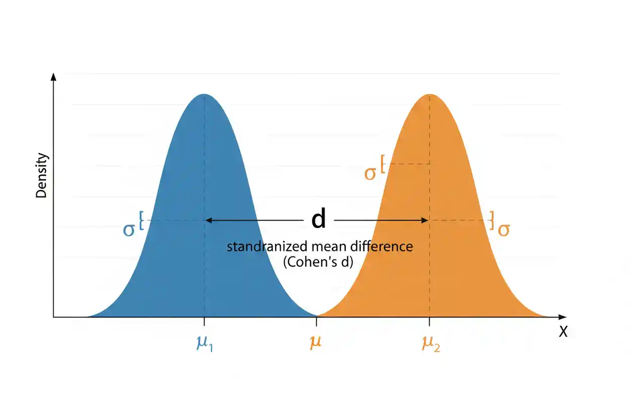

Cohen D is a standardized effect-size measure commonly used to describe the magnitude of a difference between two means. Instead of expressing a difference only in the original measurement units, Cohen’s d divides the mean difference by a relevant standard deviation, producing a dimensionless quantity that can be compared more meaningfully across measurements with different scales. For example, a 5-point difference has very different practical meaning when scores normally vary by 2 points than when they normally vary by 50 points; standardization captures that distinction.
Cohen’s d is frequently used alongside mean comparisons in experiments, observational studies, meta-analyses, and other quantitative research, but it answers a different question from a significance test. A small p-value can occur with a small standardized effect when the sample is large, while a substantial standardized effect can be estimated imprecisely in a small sample. The sign of d indicates the direction of the difference according to the order in which the group means are subtracted, while its absolute magnitude describes the separation in standard-deviation units. Interpretation should consider the subject area, measurement reliability, study design, uncertainty, and practical consequences rather than relying mechanically on universal labels such as small, medium, or large. It is also important to specify the exact version of Cohen’s d being calculated because independent-group, one-sample, and paired-data designs can require different standardization choices.
Cohen D belongs to the broader family of effect size measures used throughout Statistics & Probability. Within Inference & Regression, it complements hypothesis tests by quantifying the magnitude of a mean difference rather than merely asking whether the data provide evidence against a null hypothesis.
What Is Cohen D?
Cohen’s d expresses a mean difference relative to a standard deviation. For two independent groups, its basic form is:
d = (x̄₁ − x̄₂) / s
where x̄₁ and x̄₂ are the sample means and s is an appropriate standardizer.
When the conventional pooled-standard-deviation version is used for two independent groups:
d = (x̄₁ − x̄₂) / sₚ
where sₚ is the pooled sample standard deviation.
The result is measured in standard-deviation units rather than the original units of the variable. If:
d = 0.70
then the two sample means differ by 0.70 of the standard deviation used in the denominator.
If:
d = −0.70
the absolute standardized separation is the same, but the negative sign indicates that the first mean is lower than the second according to the subtraction order x̄₁ − x̄₂.
Cohen’s d therefore combines information about the raw mean difference with information about variability. Two studies can report the same raw difference but very different d values if their observations have different levels of dispersion.
Why Standardize a Mean Difference?
Suppose two educational programs produce mean test scores of 82 and 77. The raw difference is:
82 − 77 = 5
Whether a five-point difference is large depends heavily on how much test scores vary. If the relevant standard deviation is 5:
d = 5 / 5 = 1
The difference equals one standard deviation.
If the relevant standard deviation is instead 20:
d = 5 / 20 = 0.25
The raw five-point difference is unchanged, yet its size relative to ordinary individual variability is much smaller.
This is why standardized mean differences can be useful when comparing effects across different scales. A five-point improvement on one instrument and a three-unit improvement on another cannot ordinarily be compared directly, but standardized effects may place the differences on a more comparable dimensionless scale when the measurements and study contexts justify that comparison.
Standardization does not make fundamentally different constructs identical. A d of 0.50 in one field and d of 0.50 in another have the same mathematical standardized magnitude but may have very different substantive consequences.
Cohen D Formula for Two Independent Groups
For two independent groups under the conventional pooled-standard-deviation approach:
d = (x̄₁ − x̄₂) / sₚ
The pooled standard deviation is:
sₚ = √[((n₁ − 1)s₁² + (n₂ − 1)s₂²) / (n₁ + n₂ − 2)]
where:
- x̄₁ = mean of Group 1
- x̄₂ = mean of Group 2
- s₁ = sample standard deviation of Group 1
- s₂ = sample standard deviation of Group 2
- n₁ = sample size of Group 1
- n₂ = sample size of Group 2
- sₚ = pooled standard deviation
The pooled formula weights the two group variances by their degrees of freedom. A group with more observations therefore contributes more information to the pooled estimate than a much smaller group.
This version is most natural when the two group standard deviations can reasonably be treated as estimates of a common population standard deviation. If the population variances differ substantially, the choice of denominator deserves additional consideration rather than automatically pooling the two variances.
Worked Example: Two Independent Groups
Suppose two independent groups complete the same assessment.
Group 1 has:
n₁ = 40
x̄₁ = 78
s₁ = 10
Group 2 has:
n₂ = 40
x̄₂ = 70
s₂ = 10
Because the sample standard deviations are equal, the pooled standard deviation is also 10:
sₚ = 10
The standardized mean difference is:
d = (78 − 70) / 10
d = 8 / 10
d = 0.80
The two sample means therefore differ by 0.80 pooled standard deviations.
The raw difference is eight assessment points, while Cohen’s d describes that difference relative to the observed within-group variability. These two descriptions are complementary. The raw difference preserves the original units, while d provides a standardized measure.
Worked Example With Different Standard Deviations
Now suppose the groups have different sample standard deviations.
Group 1:
n₁ = 30
x̄₁ = 74
s₁ = 8
Group 2:
n₂ = 50
x̄₂ = 68
s₂ = 12
First calculate the pooled variance:
sₚ² = [((30 − 1) × 8²) + ((50 − 1) × 12²)] / (30 + 50 − 2)
sₚ² = [(29 × 64) + (49 × 144)] / 78
sₚ² = (1,856 + 7,056) / 78
sₚ² = 8,912 / 78
sₚ² ≈ 114.256
Now take the square root:
sₚ = √114.256
sₚ ≈ 10.689
The raw difference between the means is:
74 − 68 = 6
Therefore:
d = 6 / 10.689
d ≈ 0.561
The estimated standardized difference is approximately 0.56 pooled standard deviations.
This example also illustrates why the pooled standard deviation should not generally be obtained by simply averaging the two sample standard deviations. The pooled calculation operates on variances and accounts for sample sizes.
The Sign of Cohen D
The sign of d depends entirely on the order of subtraction.
If:
d = (x̄₁ − x̄₂) / sₚ
then a positive d means:
x̄₁ > x̄₂
while a negative d means:
x̄₁ < x̄₂
Suppose:
x̄₁ = 60
x̄₂ = 70
sₚ = 10
Then:
d = (60 − 70) / 10
d = −1
If the group order is reversed:
d = (70 − 60) / 10
d = 1
The magnitude is unchanged, but the direction reverses.
A report should therefore identify which group appears first in the subtraction. Reporting only “d = −0.60” without defining the group order can make the direction ambiguous.
Absolute Magnitude of Cohen D
When the primary interest is the size of the separation rather than its direction, researchers often discuss:
|d|
For example:
d = −0.65
has:
|d| = 0.65
The magnitude indicates a separation of 0.65 standard deviations according to the chosen denominator.
The sign should not be discarded when direction is substantively meaningful. In a treatment comparison, for instance, whether the treatment mean is above or below the control mean can be crucial. Absolute values are useful for describing magnitude, but the underlying directional information should remain available.
Common Cohen D Benchmarks
A widely repeated set of rough conventions describes:
|d| ≈ 0.20 as small
|d| ≈ 0.50 as medium
|d| ≈ 0.80 as large
These values are heuristics, not universal scientific thresholds. They were never intended to replace contextual interpretation.
A d of 0.20 could be extremely important when the outcome concerns mortality, public safety, large populations, or an inexpensive intervention with few disadvantages. A d of 0.80 could be practically trivial if the measured outcome itself has little consequence or if achieving the effect requires excessive cost or risk.
The observed distribution of effects within a particular research field is usually a better benchmark than generic labels. Researchers should therefore report the numerical value and interpret its practical meaning rather than reducing it to a category alone.
Cohen D and Effect Size
Cohen’s d is one specific standardized effect size. Effect size is a broader concept encompassing many measures of magnitude, including raw mean differences, standardized mean differences, correlations, risk ratios, odds ratios, and measures of association for categorical variables.
The correct measure depends on the type of data and research question.
Cohen’s d is particularly suited to comparisons involving means of quantitative variables. It is not the natural measure for every statistical procedure. For example, a chi-square test of independence studies association between categorical variables, where other measures of association are generally more appropriate.
Likewise, a chi-square goodness of fit test compares observed categorical frequencies with expected frequencies. Cohen’s d should not be attached automatically to such a test simply because an effect-size measure is desired.
Cohen D vs Statistical Significance
Cohen’s d measures magnitude. Statistical significance evaluates evidence against a specified null hypothesis.
These are different questions.
Suppose Study A estimates:
d = 0.20
from 20,000 observations. Because the sample is extremely large, the mean difference may be estimated with great precision and produce a very small p-value.
Study B might estimate:
d = 0.80
from only 12 observations. Despite the much larger estimated standardized effect, uncertainty could be substantial and the result might not cross a conventional significance threshold.
Therefore:
small p-value ≠ large effect
and:
large effect estimate ≠ precise effect estimate
A complete analysis should consider both magnitude and uncertainty.
The critical value used by a hypothesis test belongs to the significance-testing framework. Cohen’s d does not itself determine whether a test statistic crosses that critical boundary.
Cohen D Is Not a P-Value
A p-value and Cohen’s d cannot be interpreted interchangeably. A p-value is influenced by both effect magnitude and sampling uncertainty, including sample size. Cohen’s d primarily standardizes the observed mean difference according to the chosen measure of variability.
A result such as:
p = 0.001
does not imply:
d = 0.001
nor does:
d = 0.70
imply a 70% probability that an alternative hypothesis is correct.
They exist on entirely different scales.
This distinction is particularly important because very large samples can generate statistically significant results for effects that are small in standardized terms. Conversely, small samples may fail to produce strong inferential evidence even when the observed standardized difference is considerable.
Cohen D and the Null Hypothesis
In a typical two-group comparison, a null hypothesis may state that the population means are equal:
H₀: μ₁ − μ₂ = 0
A corresponding alternative may state:
H₁: μ₁ − μ₂ ≠ 0
Cohen’s d provides a standardized estimate of the difference represented in the sample. The significance test asks whether the observed evidence is sufficiently inconsistent with the null model according to the chosen procedure.
Rejecting H₀ does not establish that d is practically large. Failing to reject H₀ does not establish that the true standardized effect is exactly zero.
Magnitude estimation and hypothesis testing should therefore remain conceptually separate even when they are reported together.
One-Sample Cohen D
A standardized effect can also be calculated when one sample mean is compared with a fixed reference value μ₀.
A common one-sample formula is:
d = (x̄ − μ₀) / s
where x̄ is the sample mean and s is the sample standard deviation.
Suppose:
x̄ = 54
μ₀ = 50
s = 8
Then:
d = (54 − 50) / 8
d = 0.50
The sample mean is half a sample standard deviation above the reference value.
This interpretation differs structurally from a two-independent-group d because only one sample standard deviation appears in the denominator. The version used should therefore always be identified.
Cohen D for Paired Data
Paired or repeated-measures data require additional care because the two measurements are not independent. Examples include before-and-after measurements from the same participants or outcomes from matched pairs.
One common standardized mean change is based on difference scores. Let:
Dᵢ = Xafter,i − Xbefore,i
If the mean difference is D̄ and the standard deviation of the difference scores is sD, a common paired standardized effect is:
dᶻ = D̄ / sD
Suppose the mean within-person improvement is:
D̄ = 4
and the standard deviation of individual differences is:
sD = 5
Then:
dᶻ = 4 / 5
dᶻ = 0.80
This paired-data effect is not necessarily numerically equivalent to an independent-groups Cohen’s d calculated using a pooled standard deviation. The correlation between repeated measurements affects the variability of difference scores.
Several standardized-effect definitions are used for repeated-measures designs, so researchers should state the exact denominator rather than reporting an unexplained “Cohen’s d.”
Why the Denominator Matters
A standardized mean difference is only as interpretable as its standardizer. Different denominators can produce different numerical effects from the same raw mean difference.
For two independent groups, a pooled standard deviation may be appropriate under a common-variance conceptual model. In other contexts, a control-group standard deviation, difference-score standard deviation, baseline standard deviation, or another scale measure may better match the research question.
Suppose the raw difference is:
x̄₁ − x̄₂ = 6
If the denominator is 10:
d = 0.60
If the denominator is 15:
d = 0.40
The underlying six-unit mean difference has not changed. Only the scale used to standardize it has changed.
That is why effect-size reports should explain how d was computed whenever multiple definitions are plausible.
Pooled Standard Deviation vs Simple Average
The pooled standard deviation is not ordinarily:
(s₁ + s₂) / 2
Instead, it pools the group variances while accounting for their degrees of freedom:
sₚ = √[((n₁ − 1)s₁² + (n₂ − 1)s₂²) / (n₁ + n₂ − 2)]
Suppose:
n₁ = 20, s₁ = 4
and:
n₂ = 80, s₂ = 10
A simple average gives:
(4 + 10) / 2 = 7
But this treats the two standard deviations as though they contain equal amounts of information despite the second group being four times as large. The conventional pooled estimate gives greater weight to the variance estimate based on the larger group.
The distinction becomes particularly important when sample sizes or standard deviations differ substantially.
Cohen D When Variances Differ
The conventional pooled Cohen’s d assumes that combining the two group variances into a common standardizer makes substantive and statistical sense. When group variances differ greatly, that assumption may be questionable.
A pooled standardized effect can still be calculated numerically, but its interpretation may become less natural because there is no single common within-group standard deviation that clearly represents both populations.
Alternative standardized mean-difference measures use different denominators in such circumstances. The appropriate choice depends on the design and scientific question.
This issue is separate from whether a hypothesis test assumes equal variances. An analyst should not automatically choose an effect-size denominator solely because a particular testing procedure was selected.
Cohen D and Cohen’s D Notation
The measure is commonly written in prose as Cohen’s d, while tables, formulas, and software outputs often use simply:
d
The lowercase d distinguishes the standardized mean difference from many other statistical quantities.
When reporting the value, clarity is more important than stylistic variation. A statement such as:
Cohen’s d = 0.64
clearly identifies both the statistic and its estimate.
If a special form is used for paired data or another design, an additional subscript may be appropriate so that readers know how the standardization was performed.
Sample Statistic vs Population Effect
A Cohen’s d calculated from sample data is an estimate. It should not be treated as an exact population effect.
Random sampling variation affects the sample means, sample standard deviations, and therefore d itself. A new sample drawn from the same population will generally produce a different value.
The population standardized mean difference is sometimes represented using a parameter such as δ:
δ = (μ₁ − μ₂) / σ
where μ₁ and μ₂ are population means and σ is a relevant population standard deviation.
The observed Cohen’s d estimates this underlying standardized difference under the assumptions of the chosen design and estimator.
Distinguishing a sample statistic from a population parameter is especially important when the sample is small.
Small-Sample Bias
Sample Cohen’s d has a modest upward bias in estimating the absolute population standardized mean difference, particularly with small samples. In other words, its magnitude can be slightly too large on average.
A commonly used correction produces Hedges’ g by multiplying d by a factor slightly below 1:
g = Jd
One approximation to the correction factor for two independent groups is:
J ≈ 1 − 3 / [4(n₁ + n₂) − 9]
As sample size increases:
J → 1
so the difference between d and the corrected estimate becomes very small.
The important point for Cohen’s d interpretation is that its finite-sample behavior should not be ignored. A standardized effect calculated from a small sample can be both biased and highly uncertain.
Example of the Small-Sample Correction
Suppose:
d = 0.80
with:
n₁ = 10
n₂ = 10
Then:
J ≈ 1 − 3 / [4(20) − 9]
J ≈ 1 − 3/71
J ≈ 0.958
A corrected standardized effect would be approximately:
g ≈ 0.958 × 0.80
g ≈ 0.77
The correction is not enormous, but it illustrates why d should be regarded as an estimate rather than a perfect population quantity.
As the combined sample grows, the correction becomes progressively smaller.
Confidence Intervals for Cohen D
A point estimate such as:
d = 0.60
does not reveal how precisely the effect has been estimated. A confidence interval can communicate sampling uncertainty around the standardized effect.
For example, two studies might both report:
d = 0.60
but one could have an interval roughly spanning 0.45 to 0.75 while another spans −0.10 to 1.30. The point estimates are identical, but the evidence about the population effect is very different.
The precise confidence-interval calculation depends on the design, estimator, sample sizes, and assumptions. Because standardized mean differences involve estimated means and standard deviations, their sampling distributions require more than simply adding and subtracting a fixed amount from d.
Reporting uncertainty is especially valuable when sample sizes are modest.
Cohen D and Sample Size
The numerical definition of d does not contain sample size directly in its basic numerator-over-standard-deviation form, but sample size strongly affects the reliability of the estimate.
A study with:
d = 0.50
based on 1,000 observations generally estimates the population standardized difference more precisely than a study with the same d based on 12 observations, assuming comparable sampling structures.
Sample size also strongly affects statistical significance. A d of 0.20 can be highly statistically significant in a very large study, while d = 0.80 can remain uncertain in a very small one.
This reinforces the distinction between effect magnitude and inferential precision.
Cohen D and Statistical Power
Power depends partly on the effect size that a study is designed to detect. All else equal, larger standardized mean differences are easier to distinguish from zero than smaller ones.
For example, detecting:
d = 0.80
usually requires fewer observations than detecting:
d = 0.20
at the same significance level and desired statistical power under a comparable two-group design.
However, observed Cohen’s d should not be treated as a guaranteed true effect for future power calculations. Estimates from small studies can be unstable and may overstate the underlying magnitude.
Planning decisions should therefore consider prior evidence, realistic minimum effects of interest, and uncertainty rather than relying uncritically on one observed d.
Cohen D vs Coefficient of Determination
The coefficient of determination and Cohen’s d are both dimensionless statistical measures, but they describe different aspects of data.
Cohen’s d standardizes a difference between means:
d = mean difference / standard deviation
The coefficient of determination, R², describes how much variation in a response is represented by a regression model relative to a baseline.
An R² of 0.50 does not mean the same thing as:
d = 0.50
The values should not be compared as though they lie on a common substantive scale.
A statistical analysis should use the measure that corresponds to the structure of the question rather than whichever number appears more familiar.
Cohen D vs Chi-Square Tests
Cohen’s d is designed for standardized differences involving quantitative outcomes. Chi-square procedures generally operate on categorical frequency counts.
The chi-square test of independence asks whether two categorical variables are associated. The chi-square goodness of fit test asks whether one categorical distribution matches specified expected probabilities.
Neither procedure naturally produces Cohen’s d from its chi-square statistic alone.
A statistically significant chi-square result therefore should not be converted casually into d without a valid mathematical relationship and a research question for which standardized mean differences are meaningful.
Raw Mean Difference vs Cohen D
A raw mean difference preserves the original measurement units:
Difference = x̄₁ − x̄₂
Cohen’s d standardizes the same difference:
d = (x̄₁ − x̄₂) / s
Each measure provides useful but different information.
Suppose a treatment reduces average processing time by:
3 minutes
and:
d = 0.75
The three-minute figure is directly interpretable in operational terms. The d value indicates that the mean difference corresponds to three-quarters of the chosen standard deviation.
A strong report often includes both. Standardized measures improve comparability, while raw differences preserve practical meaning.
What Does d = 0 Mean?
If:
d = 0
then the two sample means are equal under the relevant formula:
x̄₁ = x̄₂
provided the denominator is positive and finite.
This does not mean the two distributions are identical. The groups could have equal means while differing in variance, skewness, shape, or other properties.
Cohen’s d summarizes a standardized difference in means. It is not a general-purpose measure of every possible difference between distributions.
Can Cohen D Be Greater Than 1?
Yes. Cohen’s d is not limited to the interval from −1 to 1.
For example, if:
x̄₁ − x̄₂ = 18
and:
sₚ = 10
then:
d = 18/10
d = 1.80
The group means differ by 1.8 pooled standard deviations.
Values above 1 or below −1 are mathematically valid and can occur when group means are widely separated relative to within-group variability.
There is no theoretical upper or lower bound comparable to a correlation coefficient’s −1 to 1 range.
Can Cohen D Be Negative?
Yes. A negative Cohen’s d simply indicates direction under the chosen group ordering.
Suppose:
x̄₁ = 45
x̄₂ = 50
sₚ = 10
Then:
d = (45 − 50) / 10
d = −0.50
Group 1 is half a pooled standard deviation below Group 2.
If the labels are reversed, the result becomes +0.50. The effect magnitude is unchanged.
Influence of Outliers
Cohen’s d is built from means and standard deviations, both of which can be sensitive to extreme observations. An outlier can alter the numerator by shifting a group mean, the denominator by increasing a group standard deviation, or both.
As a result, a single unusual observation can sometimes change d substantially in a small sample.
Before interpreting the standardized effect, researchers should examine the data distribution and determine whether extreme values are genuine observations, measurement errors, or evidence that a mean-and-standard-deviation summary is poorly suited to the outcome.
Deleting observations solely because they weaken or strengthen d is not appropriate. Any data-quality decision should follow defensible criteria independent of the desired result.
Non-Normal Data
The formula for Cohen’s d can be calculated even when observations are not perfectly normally distributed. Normality is not an algebraic requirement for subtracting means and dividing by a standard deviation.
However, severe skewness, heavy tails, or extreme outliers can make the mean and standard deviation less representative of the typical distribution. They can also affect inferential procedures used to construct confidence intervals or test hypotheses.
The substantive usefulness of d therefore depends on whether a standardized mean difference is a meaningful description of the data.
A distribution should not be assumed appropriate for mean-based summaries merely because d can be computed numerically.
Interpreting Cohen D in Overlapping Distributions
Cohen’s d is sometimes explained visually using two distributions with equal standard deviations. A larger absolute d corresponds to greater separation between their means relative to their spread.
At:
d = 0
the means coincide.
At:
|d| = 0.50
the means are separated by half a standard deviation.
At:
|d| = 1
the means are separated by one standard deviation.
This visualization can be useful, but it assumes a simplified distributional picture. Real groups can differ in variance, skewness, modality, and other features. Cohen’s d alone cannot describe those differences.
It should therefore be understood as a standardized mean-separation measure rather than a complete measure of distributional overlap.
Practical Example: Employee Training
Suppose a company evaluates a training program using a performance score. The trained group has:
n₁ = 60
x̄₁ = 84
s₁ = 12
The comparison group has:
n₂ = 60
x̄₂ = 78
s₂ = 12
The pooled standard deviation is:
sₚ = 12
Therefore:
d = (84 − 78) / 12
d = 6/12
d = 0.50
The standardized difference is half a standard deviation.
The raw six-point difference may be more important operationally if managers understand the scoring scale directly. Cohen’s d adds another perspective by showing that six points correspond to one-half of the observed within-group variability.
Whether that effect justifies the training program depends on factors such as cost, persistence of the improvement, measurement reliability, and the relationship between score changes and actual job performance.
Practical Example: Medical Measurement
Suppose a treatment group has an average reduction in a quantitative measurement of 7 units, while the control group averages a reduction of 3 units. If the pooled standard deviation is 8:
d = (7 − 3) / 8
d = 4/8
d = 0.50
The standardized difference is again 0.50.
That numerical value does not determine whether the treatment effect is medically important. Four units may be clinically transformative or essentially irrelevant depending on the outcome.
Statistical standardization cannot replace subject-matter judgment.
Common Mistakes
A common mistake is interpreting Cohen’s d as the percentage of participants who improved. A value such as:
d = 0.60
does not mean 60% improved. It represents a mean difference equal to 0.60 of the chosen standard deviation.
Another error is treating d as a probability. A d of 0.80 does not mean there is an 80% probability that one treatment is superior.
Researchers also sometimes report d without identifying the group order. Because changing the subtraction order changes the sign, the direction can become ambiguous.
A further mistake is mixing formulas for independent and paired data. Standardizing a paired mean difference by the standard deviation of difference scores is not the same calculation as pooling two independent-group standard deviations.
Finally, universal benchmark labels should not replace substantive interpretation. The consequences associated with an effect matter more than whether a number happens to exceed 0.20, 0.50, or 0.80.
How to Calculate Cohen D
For two independent groups using the conventional pooled standard deviation, first identify:
x̄₁, x̄₂, s₁, s₂, n₁, n₂
Calculate the pooled standard deviation:
sₚ = √[((n₁ − 1)s₁² + (n₂ − 1)s₂²) / (n₁ + n₂ − 2)]
Then calculate the raw mean difference:
Δx̄ = x̄₁ − x̄₂
Finally standardize it:
d = Δx̄ / sₚ
Report both the value and direction, and state which group was subtracted from which.
Before applying the formula mechanically, verify that the independent-group pooled-standard-deviation version matches the study design.
How to Report Cohen D
A concise report might state:
Group 1 scored higher than Group 2 by 6 points, corresponding to Cohen’s d = 0.56 using the pooled standard deviation.
This communicates the raw difference, standardized magnitude, direction, and denominator convention.
When uncertainty estimates are available, they can be reported as well. An effect-size confidence interval often gives readers substantially more information than a point estimate alone.
If the study uses paired observations, a one-sample design, or another special standardizer, that version should be named so the result can be interpreted and reproduced correctly.
Frequently Asked Questions
What is Cohen D?
Cohen’s d is a standardized mean-difference measure. It expresses the difference between means relative to a relevant standard deviation.
What is the basic Cohen D formula?
For two independent groups using a pooled standard deviation:
d = (x̄₁ − x̄₂) / sₚ
where sₚ is the pooled sample standard deviation.
How do you calculate the pooled standard deviation?
The conventional formula is:
sₚ = √[((n₁ − 1)s₁² + (n₂ − 1)s₂²) / (n₁ + n₂ − 2)]
It weights the group variances according to their degrees of freedom.
What does Cohen D = 0.5 mean?
It means the group means differ by one-half of the standard deviation used to standardize the difference.
Is Cohen D = 0.5 always a medium effect?
It is often labeled medium under a traditional rule of thumb, but that label is not universal. Practical importance depends on the research context.
What does a negative Cohen D mean?
A negative value indicates that the first mean in the subtraction is lower than the second. Reversing the group order reverses the sign.
Can Cohen D be greater than 1?
Yes. Cohen’s d has no theoretical restriction to −1 through 1. A value of 1.5 means the means differ by 1.5 standard deviations according to the chosen standardizer.
Is Cohen D the same as statistical significance?
No. Cohen’s d measures standardized effect magnitude. Statistical significance evaluates evidence against a null hypothesis and is strongly affected by sample size and uncertainty.
Is Cohen D a p-value?
No. The measures have completely different definitions and interpretations.
Does Cohen D prove causation?
No. A standardized mean difference describes an observed magnitude. Whether the difference can be interpreted causally depends on the research design and assumptions.
Can Cohen D be used with paired data?
Yes, but paired designs require an appropriate paired-effect definition. A common version divides the mean difference score by the standard deviation of the difference scores.
Can Cohen D be used for one sample?
Yes. One common formula is:
d = (x̄ − μ₀) / s
where μ₀ is the reference value.
Is Cohen D biased in small samples?
The sample estimate has some small-sample bias in magnitude. Hedges’ g applies a correction that becomes increasingly minor as sample size grows.
Should Cohen D be reported with a confidence interval?
When possible, yes. A confidence interval communicates uncertainty around the standardized effect rather than presenting the point estimate as exact.
Is Cohen D appropriate for categorical variables?
Usually not. Cohen’s d is designed for standardized differences involving quantitative measurements. Categorical-frequency problems generally require other association or effect-size measures.
Key Takeaway
Cohen D measures the size of a mean difference relative to a relevant standard deviation. For two independent groups under the conventional pooled approach:
d = (x̄₁ − x̄₂) / sₚ
with:
sₚ = √[((n₁ − 1)s₁² + (n₂ − 1)s₂²) / (n₁ + n₂ − 2)]
The sign indicates direction, while the absolute value represents standardized magnitude. A d of 0.50 means the means differ by half of the standard deviation used in the calculation; it does not mean a 50% improvement, 50% accuracy, or a 50% probability of an effect. Cohen’s d should also remain separate from statistical significance: sample size and uncertainty affect hypothesis-test results, while d primarily describes standardized magnitude. Its interpretation is strongest when the raw mean difference, calculation method, confidence interval, study design, and practical consequences are considered together rather than reducing the result to a universal small, medium, or large label.



