
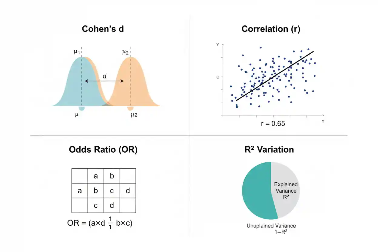

Effect size is a numerical measure of how large a difference, relationship, association, or model contribution is, rather than merely whether statistical evidence against a null hypothesis exists. It helps answer questions such as how far apart two group means are, how strongly two variables are related, how much variation a model accounts for, or how much more likely an outcome is in one group than another. This makes effect size fundamentally different from statistical significance. A very small effect can produce a small p-value when the sample is sufficiently large, while a substantial estimated effect can remain statistically uncertain when a study contains little information. Effect sizes can be expressed in original measurement units, standardized units, proportions, correlations, ratios, or other scales depending on the data and research question.
No single formula therefore represents every effect size. A standardized mean difference such as Cohen D is appropriate for some group comparisons, while regression, categorical, binary-outcome, and correlational analyses use different measures. Correct interpretation also requires uncertainty, study design, baseline risk, measurement quality, and practical consequences to be considered. The numerical magnitude is valuable because it describes the size of an observed phenomenon, but that magnitude should never be separated from the context that gives it meaning.
Effect sizes are a core part of Statistics & Probability and especially important within Inference & Regression, where estimation, uncertainty, hypothesis testing, and practical interpretation need to remain distinct.
What Is Effect Size?
An effect size is a statistic or parameter that quantifies the magnitude of a phenomenon of interest. Depending on the analysis, that phenomenon might be a difference between two means, a relationship between quantitative variables, an association between categorical outcomes, a change in risk, or the proportion of variation represented by a statistical model.
The key idea is magnitude.
Suppose two groups have means of 75 and 70. The raw difference is:
Mean difference = 75 − 70 = 5
That five-unit difference is itself an effect size because it quantifies how far apart the group means are in the original measurement units.
If the relevant within-group standard deviation is 10, the same difference can be standardized:
Standardized mean difference = 5 / 10 = 0.50
Now the effect is expressed as one-half of a standard deviation rather than five original units.
Neither representation is inherently superior. The raw difference is often easier to interpret practically, while the standardized difference can make comparison across different measurement scales easier.
Why Effect Size Matters
A statistical analysis should usually answer more than whether an observed pattern is inconsistent with a particular null model. Researchers, analysts, and decision-makers generally care about how large the pattern is.
Suppose an enormous study compares two groups and finds average values of:
Group 1 mean = 100.0
Group 2 mean = 100.3
The raw effect is only:
100.3 − 100.0 = 0.3
With hundreds of thousands of observations, that tiny difference could potentially produce very strong statistical evidence against equality of population means. Yet a difference of 0.3 units may have little practical consequence.
Now imagine a much smaller study finds a 12-unit difference but estimates it imprecisely. The result may not cross a conventional significance threshold even though the observed magnitude is large.
These examples illustrate why effect magnitude and inferential evidence must be considered separately. Statistical significance asks whether the data are sufficiently inconsistent with a particular null hypothesis under a defined testing procedure. Effect size describes how large the observed or estimated phenomenon is.
Effect Size vs Statistical Significance
Statistical significance is largely a statement about compatibility between sample evidence and a null model. Effect size is a statement about magnitude.
The two can move differently because significance depends strongly on precision, which in turn depends on quantities such as sample size, variability, and study design.
Consider two hypothetical studies.
Study A reports:
Standardized effect = 0.15
with a very large sample.
Study B reports:
Standardized effect = 0.75
with a very small sample.
Study A may produce a much smaller p-value because its estimate is extremely precise, even though the effect itself is smaller. Study B may produce weaker evidence because its estimate is uncertain despite its larger observed magnitude.
Therefore:
statistical significance ≠ effect magnitude
and:
statistical insignificance ≠ zero effect
A good interpretation reports the effect itself, its uncertainty, and the inferential evidence rather than reducing the entire analysis to whether a threshold was crossed.
The threshold used in a significance test may depend on a Critical Value, but the critical value does not describe the size or practical importance of the underlying phenomenon.
Absolute and Standardized Effect Sizes
Effect sizes can be divided broadly into absolute and standardized measures.
An absolute effect remains in meaningful original units. For two group means:
Raw mean difference = x̄₁ − x̄₂
If average recovery time is 18 days for one treatment and 22 days for another:
Difference = 18 − 22 = −4 days
The magnitude is four days.
A standardized effect divides a raw difference or relationship by an appropriate scale so that the result is dimensionless. For example:
d = (x̄₁ − x̄₂) / s
where s is an appropriate standard deviation.
Standardized effects can facilitate comparison across instruments or studies, but the original-unit effect often remains more directly useful for practical decisions.
An effective statistical report frequently includes both when each contributes distinct information.
Raw Mean Difference as an Effect Size
The simplest effect size for comparing two quantitative group means is often the raw mean difference:
Δ = x̄₁ − x̄₂
Suppose a new process takes an average of 42 minutes while the existing process takes 50 minutes:
Δ = 42 − 50
Δ = −8 minutes
The new process is associated with an eight-minute lower average completion time in the sample.
This result is immediately interpretable because the outcome remains in minutes. Managers can compare eight minutes with staffing costs, production volumes, service-level targets, or other operational considerations.
The limitation is comparability across scales. An eight-unit difference in minutes cannot be directly compared with an eight-unit difference in a psychological score, blood-pressure measure, or financial index. Standardization can help when cross-scale comparison is genuinely useful.
Standardized Mean Difference
A standardized mean difference expresses a difference in standard-deviation units. A generic form is:
Standardized mean difference = Mean difference / relevant standard deviation
One familiar version is Cohen D, which for two independent groups under the conventional pooled-standard-deviation approach is:
d = (x̄₁ − x̄₂) / sₚ
Suppose:
x̄₁ = 82
x̄₂ = 74
sₚ = 10
Then:
d = (82 − 74) / 10
d = 0.80
The means differ by 0.80 pooled standard deviations.
This does not mean an 80% improvement, 80% accuracy, or an 80% probability that one group is better. It is a standardized distance between the two means.
Worked Example: Raw and Standardized Effects
Suppose two training methods are compared using an assessment scored from 0 to 100.
Method A:
x̄A = 78
Method B:
x̄B = 72
The raw mean difference is:
Δ = 78 − 72
Δ = 6 points
Assume the pooled standard deviation is:
sₚ = 12
The standardized mean difference is:
d = 6 / 12
d = 0.50
Both statistics describe the same observed group difference from different perspectives. The six-point raw difference preserves the original assessment scale. The standardized value shows that those six points correspond to half of the pooled standard deviation.
Whether the effect is important depends on what a six-point improvement means in practice. If six points move participants across an important competency threshold, the effect could be highly consequential. If the score is noisy and six points have no operational meaning, the same standardized magnitude may matter much less.
Correlation as an Effect Size
A correlation coefficient can serve as an effect-size measure for the strength and direction of a relationship between two quantitative variables.
Pearson’s correlation coefficient is commonly written:
r = covariance(X,Y) / (sₓsᵧ)
Its familiar range is:
−1 ≤ r ≤ 1
A positive value indicates a positive linear relationship, a negative value indicates a negative linear relationship, and a value near zero indicates little linear association.
For example:
r = 0.70
indicates a stronger positive linear relationship than:
r = 0.15
in the usual descriptive sense.
The sign matters because it communicates direction. Unlike a standardized mean difference where researchers sometimes focus on absolute magnitude, reversing the sign of a correlation changes the direction of the relationship.
Correlation still does not imply causation. A large |r| can arise because of direct causation, reverse causation, confounding, common trends, selection, or other structures.
R² as a Measure of Model Fit Magnitude
Regression analysis often uses the Coefficient Of Determination, R², to describe how much variation in an outcome is represented by a fitted model relative to a baseline.
Under the conventional ordinary least squares formulation:
R² = 1 − SSE / SST
where SSE is the residual sum of squares and SST is the total sum of squares.
Suppose:
SSE = 300
and:
SST = 1,000
Then:
R² = 1 − 300/1,000
R² = 0.70
The model accounts for 70% of the observed variation relative to the relevant mean-based baseline in this conventional setting.
R² is dimensionless, but it should not be confused with a standardized mean difference. An R² of 0.50 and a d of 0.50 have completely different mathematical meanings.
Effect Size in Multiple Regression
In Multiple Regression, effect magnitude can be described at several levels. The overall model may be summarized using measures such as R², while individual regression coefficients describe the estimated change in the response associated with a predictor when the other included predictors are held constant under the model.
A generic multiple linear regression model can be expressed as:
ŷ = b₀ + b₁x₁ + b₂x₂ + … + bₖxₖ
The coefficient b₁ is an effect estimate on the original outcome scale if x₁ changes by one unit while the other included predictors remain fixed.
For example:
b₁ = 4.5
might indicate an estimated 4.5-unit difference in the response per one-unit increase in x₁, conditional on the other predictors in the model.
This coefficient can be substantively meaningful even if the overall R² is modest. Conversely, a model can have high R² while an individual predictor contributes little unique information.
Effect size should therefore correspond to the specific question being asked: overall fit and individual predictor magnitude are different quantities.
Effect Size in Logistic Regression
When an outcome is binary, Logistic Regression models the log-odds of the outcome rather than the outcome directly as an unrestricted linear quantity.
A basic form is:
log[p / (1 − p)] = β₀ + β₁x
Exponentiating a coefficient gives an odds ratio:
OR = e^β¹
Suppose:
β₁ = 0.693
Then:
OR ≈ e^0.693
OR ≈ 2
Under the model, a one-unit increase in x is associated with approximately twice the odds of the outcome, holding relevant included predictors constant.
An odds ratio is therefore another form of effect measure. Its interpretation differs substantially from Cohen’s d, a raw mean difference, correlation, or R².
The existence of several valid effect metrics is exactly why the phrase effect size must always be tied to the type of outcome and statistical model.
Risk Difference
For binary outcomes, one direct measure of magnitude is the risk difference.
Suppose:
Risk in Group 1 = p₁
Risk in Group 2 = p₂
Then:
Risk difference = p₁ − p₂
If:
p₁ = 0.30
and:
p₂ = 0.20
then:
Risk difference = 0.30 − 0.20
Risk difference = 0.10
The absolute difference is 0.10, or 10 percentage points.
This measure is often intuitively useful because it remains on the probability scale. If the outcome is undesirable, a reduction from 30% to 20% means 10 fewer events per 100 comparable individuals under a simple descriptive interpretation.
As with other observational effect estimates, causal language requires a design capable of supporting it.
Risk Ratio
Another binary-outcome effect size is the risk ratio:
RR = p₁ / p₂
If:
p₁ = 0.30
and:
p₂ = 0.20
then:
RR = 0.30 / 0.20
RR = 1.5
The risk in Group 1 is 1.5 times the risk in Group 2.
A risk ratio is a relative effect, whereas the risk difference is an absolute effect. The two provide complementary information.
A change from 1% to 2% gives:
RR = 2
but only a one-percentage-point absolute increase.
A change from 20% to 40% also gives:
RR = 2
but represents a 20-percentage-point absolute increase.
This illustrates why relative effect measures should often be considered alongside absolute risks.
Odds Ratio
An odds ratio compares odds rather than probabilities.
If an event has probability p, its odds are:
Odds = p / (1 − p)
For two groups:
OR = [p₁ / (1 − p₁)] / [p₂ / (1 − p₂)]
Suppose:
p₁ = 0.40
and:
p₂ = 0.20
Then:
Odds₁ = 0.40 / 0.60 ≈ 0.667
Odds₂ = 0.20 / 0.80 = 0.25
Therefore:
OR ≈ 0.667 / 0.25
OR ≈ 2.67
Notice that the risk ratio is:
RR = 0.40 / 0.20 = 2
The odds ratio and risk ratio are therefore not generally equal. When outcomes are uncommon, they can be numerically similar; when outcomes are common, the difference can become substantial.
An odds ratio should not automatically be described as a risk ratio.
Relative vs Absolute Effect Size
Relative and absolute effect sizes answer different practical questions.
Suppose a treatment lowers the probability of an event from:
2% to 1%
The absolute risk reduction is:
0.02 − 0.01 = 0.01
or one percentage point.
The relative risk is:
0.01 / 0.02 = 0.50
so the treated risk is half the comparison risk.
Now consider a reduction from:
40% to 20%
The relative risk is again:
0.20 / 0.40 = 0.50
but the absolute risk reduction is:
0.40 − 0.20 = 0.20
or 20 percentage points.
The same relative effect can therefore correspond to dramatically different absolute consequences. Decision-making often benefits from seeing both.
Direction of an Effect
Some effect-size measures carry directional information.
For a raw mean difference:
x̄₁ − x̄₂
a positive result indicates that Group 1 has the larger mean, while a negative result indicates that Group 1 has the smaller mean.
For Cohen’s d, the sign similarly follows the subtraction order.
For correlation:
r > 0
indicates a positive relationship, whereas:
r < 0
indicates a negative relationship.
Ratio measures behave differently. For a risk ratio or odds ratio:
ratio = 1
represents the natural null value.
Values above 1 indicate greater relative risk or odds in the numerator group, while values below 1 indicate lower relative risk or odds.
The natural reference point therefore depends on the effect metric.
Null Values for Common Effect Sizes
Different effect-size measures have different values representing no effect.
For a mean difference:
Null value = 0
For Cohen’s d:
Null value = 0
For correlation:
Null value = 0
For a regression coefficient testing no linear contribution:
Null value = 0
For a risk difference:
Null value = 0
For risk ratios and odds ratios:
Null value = 1
For R² in the conventional model-fit interpretation, 0 represents no improvement in squared-error fit over the baseline, but its role differs from a null effect parameter in a simple group comparison.
Knowing the natural null value is essential when interpreting confidence intervals and inferential tests.
Confidence Intervals for Effect Sizes
An effect-size point estimate does not reveal its precision. Confidence intervals provide information about the range of parameter values compatible with the data under a specified repeated-sampling procedure and model assumptions.
Suppose an estimated standardized effect is:
d = 0.50
An interval might be:
0.10 to 0.90
This indicates substantial uncertainty about the exact population magnitude even though the point estimate is 0.50.
Another study might estimate the same:
d = 0.50
with an interval:
0.45 to 0.55
The point estimates are identical, but the second study provides much greater precision.
A frequentist 95% confidence interval should not be interpreted as meaning there is a 95% posterior probability that the fixed population effect lies between the observed endpoints. Its 95% property concerns the long-run coverage of the interval-producing procedure under its assumptions.
Statistical Significance From an Effect Interval
For many common effect estimands, confidence intervals can indicate whether a corresponding null value is excluded.
If a mean difference has a 95% interval:
2.1 to 8.4
zero is excluded.
If an odds ratio has a 95% interval:
1.20 to 2.10
one is excluded.
These results typically align with a corresponding two-sided test at α = 0.05 when the interval and hypothesis test are constructed from compatible methods.
However, exclusion of the null value does not establish practical importance. An extremely narrow interval around a tiny nonzero effect can be statistically persuasive but substantively trivial.
The interval should be interpreted for both whether it excludes the null and what effect magnitudes it still permits.
Practical Significance
Practical significance asks whether an effect is large enough to matter in the real decision environment.
Suppose a new process saves:
0.2 seconds per transaction
If only 50 transactions occur each month, the effect may be operationally irrelevant.
If billions of transactions occur, the same per-transaction effect could accumulate into substantial resource savings.
Likewise, a very small average change in a medical outcome can have major public-health implications when applied across a large population, while a statistically impressive change in a laboratory surrogate may have little effect on outcomes people actually care about.
Practical importance therefore cannot be determined from a universal numerical threshold alone.
Clinical and Operational Importance
In applied fields, analysts sometimes define a minimum effect that would justify changing practice. This may be referred to as a minimum clinically important difference, minimum practically important difference, or minimum effect of interest depending on context.
Suppose a new intervention costs substantially more than an existing one. Decision-makers may conclude that an improvement smaller than five units is not worth the added expense.
An estimated effect of:
1.5 units
could be statistically significant with enough data but remain below the five-unit practical threshold.
Conversely, an estimated effect of:
7 units
with substantial uncertainty might be practically promising even if the current study is too small for a definitive inferential conclusion.
Explicit practical thresholds can make interpretation more decision-relevant than vague labels such as “significant.”
Small, Medium, and Large Effects
Standardized effect sizes are often interpreted with conventional labels. For Cohen’s d, frequently cited heuristics include approximately:
0.20 = small
0.50 = medium
0.80 = large
These are broad conventions rather than laws.
For correlations, other rough conventions are sometimes used, but the same caution applies. An r that is considered small in one field may be highly consequential in another.
The best benchmark often comes from the distribution of effects in the relevant discipline, the reliability of the measurement, the costs and benefits of decisions, and the minimum magnitude that would change practice.
A numerical estimate should therefore be reported directly rather than replaced by a verbal label.
Why Context Changes Effect-Size Interpretation
Suppose a standardized effect is:
d = 0.25
In a low-cost educational intervention delivered automatically to millions of students, that effect may be extremely valuable.
The same d = 0.25 for an invasive, expensive procedure with serious adverse effects may be unacceptable.
Similarly, a correlation of:
r = 0.20
could be practically useful for forecasting a high-volume phenomenon when combined with other information, yet inadequate for making a high-stakes individual decision.
Effect magnitude acquires meaning only after the decision context, costs, risks, and alternatives are considered.
Sample Effect Size vs Population Effect
An effect calculated from a sample is generally a statistic that estimates an unknown population quantity.
Suppose a sample gives:
d = 0.60
A different random sample from the same population will usually produce a different d because the sample means and standard deviations change.
The same applies to:
r
R²
odds ratios
risk ratios
and regression coefficients.
Observed effect sizes therefore contain sampling variability. The point estimate is not the population truth simply because it has been calculated to several decimal places.
Confidence intervals, repeated studies, replication, and model validation help quantify or reveal this uncertainty.
Sample Size and Effect Size
Increasing sample size does not necessarily make the underlying population effect larger. Instead, larger samples generally allow an effect to be estimated more precisely.
Suppose the true standardized effect is approximately:
δ = 0.30
A sample of 20 observations may produce:
d = 0.05
or:
d = 0.70
simply because sampling variability is large.
A much larger study is more likely to produce an estimate relatively close to the population value, assuming the sampling design and measurement process are sound.
At the same time, increasing sample size makes even small effects easier to distinguish statistically from the null. This is why very large studies can produce small p-values for effects of minor practical importance.
Effect Size and Statistical Power
Statistical power is the probability that a testing procedure rejects H₀ under a specified alternative effect and set of assumptions.
Larger true effects are generally easier to detect than smaller effects when sample size, variability, significance level, and design remain otherwise comparable.
For example, a study designed to detect:
d = 0.80
usually requires fewer observations than one designed to reliably detect:
d = 0.20
under the same basic two-group framework.
Effect size is therefore a central input into sample-size and power planning.
However, using an unstable effect estimate from a very small previous study can lead to unrealistic planning. Observed effects are subject to sampling variation and, in selective literatures, publication and selection biases.
Measurement Reliability and Effect Size
Measurement error can influence observed effect magnitudes. If an outcome measure contains substantial random noise, the variance may increase while stable differences or associations become harder to detect.
For standardized mean differences, greater unexplained measurement variability can enlarge the denominator and reduce the observed standardized effect.
For correlations, unreliability can attenuate observed relationships.
This does not mean an analyst should simply “correct” every observed statistic without strong assumptions. It means effect-size interpretation should consider whether the measurement system is sufficiently reliable for the research question.
A precise-looking numerical effect based on a poor measurement instrument can be less informative than a somewhat uncertain effect obtained from a valid and reliable measure.
Outliers and Effect Size
Some effect-size measures are sensitive to extreme observations because they depend on means, standard deviations, correlations, or model coefficients.
For example, one extreme value can shift a group mean and substantially increase its standard deviation. The resulting Cohen’s d may move upward or downward depending on how both numerator and denominator change.
Pearson correlation can also be heavily influenced by unusual observations.
Regression-based effect measures may change substantially if high-leverage points influence the fitted model.
Effect size should therefore be interpreted after examining whether the data contain influential observations and whether those observations are genuine, erroneous, or evidence that a different model is needed.
Deleting inconvenient observations merely to increase or decrease the reported effect is not valid analysis.
Effect Size and Skewed Data
Standardized mean differences are often easiest to interpret when means and standard deviations provide meaningful summaries of the distributions involved.
With severe skewness or heavy tails, those summaries may become less representative of typical observations. Two groups can have the same mean difference but very different distributional shapes.
Likewise, a correlation coefficient focused on linear association can miss a strong nonlinear relationship.
The appropriate effect-size measure should match the structure of the data. Numerical calculation alone does not guarantee meaningful interpretation.
Effect Size Does Not Establish Causation
An effect size can be large even when the relationship is noncausal.
Suppose an observational dataset shows a large difference between two groups. The difference might reflect the group-defining exposure, but it might also result from confounding, self-selection, reverse causality, measurement differences, or omitted variables.
Similarly, a large regression coefficient or odds ratio does not become causal merely because it is statistically precise.
Causal interpretation requires a research design and assumptions that justify causal identification.
Effect size answers “how large is the observed or modeled relationship?” Causal inference asks a different question: “what would change if an intervention changed the exposure while relevant alternative explanations were appropriately addressed?”
Effect Size and Model Fit Are Not the Same
Some measures, such as R², summarize an aspect of overall model fit and can function as magnitude measures in that context. Other effect sizes describe individual parameters.
Suppose a multiple regression has:
R² = 0.75
but a particular predictor has a coefficient very close to zero after adjustment for other variables.
The model can fit the outcome well overall while that individual predictor contributes little unique conditional association.
Conversely, an important predictor can have a meaningful coefficient in a noisy outcome where overall R² remains low.
Effect size must therefore be attached to a clearly defined estimand: overall model performance and individual predictor effects should not be conflated.
Choosing the Right Effect Size
The most appropriate effect measure follows from the research question and data structure.
If the question concerns a difference between quantitative means, a raw mean difference or standardized mean difference may be appropriate.
If it concerns a linear relationship between two quantitative variables, a correlation may be useful.
If the outcome is binary, a risk difference, risk ratio, or odds ratio may be relevant depending on the objective and study design.
If the question concerns regression model fit, R² may provide useful information in an appropriate model.
If the focus is an individual regression coefficient, the coefficient itself may be the meaningful effect estimate, potentially accompanied by a standardized version when comparison across predictors is justified.
There is no universal effect-size statistic that should be attached to every analysis.
Worked Example: Same Significance, Different Effects
Imagine two independent studies both return p ≈ 0.04.
Study A estimates:
d = 0.15
Study B estimates:
d = 0.75
The same approximate p-value does not imply the same effect magnitude.
Study A may contain a large sample that allows a small effect to be estimated precisely. Study B may contain a smaller sample and a larger but less precise effect.
Reporting only “p < 0.05” would hide this substantial difference.
Effect estimates reveal information that significance decisions cannot provide.
Worked Example: Same Effect, Different Precision
Now suppose two studies both estimate:
d = 0.50
Study A has a very small sample and a wide confidence interval.
Study B contains many more observations and has a narrow confidence interval.
The point effect is identical, but the certainty about the underlying population effect is not.
This distinction shows why even effect size alone is not sufficient. Magnitude and uncertainty must be reported together whenever the inferential objective extends beyond the observed sample.
Effect Size and Confidence Interval Width
Confidence interval width depends on precision. Larger samples, lower variability, and efficient research designs generally produce narrower intervals.
Suppose one study reports:
d = 0.40, 95% CI approximately −0.15 to 0.95
Another reports:
d = 0.40, 95% CI approximately 0.33 to 0.47
The first study is compatible with effects ranging from moderately negative to substantially positive. The second provides much more precise evidence for a positive effect near 0.40.
A point estimate should therefore never be interpreted as though all nearby or alternative values have been ruled out.
Effect Size in Meta-Analysis
Standardized effect sizes are particularly useful when results from different studies need to be synthesized but the studies use different measurement scales.
For example, several studies might measure a similar construct using different validated instruments. Raw point differences cannot be pooled directly when the scales differ, whereas appropriately defined standardized mean differences can sometimes place the effects onto a common metric.
The same principle applies to logarithms of ratio measures and other transformation-based meta-analytic metrics.
However, statistical standardization does not make substantively different constructs equivalent. Combining studies still requires that their populations, interventions, outcomes, and designs be sufficiently comparable for the pooled question to make sense.
Effect Size and Units
One advantage of standardized measures is that they remove the original measurement units.
For:
d = 0.50
the value does not carry units such as kilograms, dollars, seconds, or test points.
This helps comparison but also removes some direct practical meaning.
A raw difference such as:
−8 minutes
is immediately understandable.
A standardized value such as:
d = −0.65
requires knowledge of the reference variability before its practical meaning becomes intuitive.
For that reason, standardized and unstandardized effects often complement one another rather than compete.
Common Misconceptions About Effect Size
A common misconception is that effect size and statistical significance are interchangeable. They are not. Magnitude and inferential evidence answer different questions.
Another mistake is assuming standardized effect values are percentages. A Cohen’s d of 0.60 is not a 60% difference. It means the means are separated by 0.60 of the standard deviation used in the calculation.
A third mistake is assuming that a large effect proves causation. Effect magnitude says nothing by itself about whether an association is causal.
Another error is using one universal threshold for every discipline. A numerically small effect can have major real-world consequences, while a large standardized effect can be practically unimportant.
Researchers also sometimes compare effect measures that use different scales as if their numerical values were directly interchangeable. An R² of 0.40, a correlation of 0.40, Cohen’s d of 0.40, and an odds ratio of 0.40 do not represent the same magnitude.
Finally, an effect-size estimate should not be treated as exact. Sampling uncertainty remains important.
How to Interpret an Effect Size Properly
Begin by identifying exactly what the statistic measures. Determine whether the effect represents a mean difference, standardized difference, association, probability difference, ratio, regression coefficient, or model-fit quantity.
Next identify its null or reference value. For differences and many coefficients, that value is often zero. For ratios, it is usually one.
Then consider direction and scale. Ask what a positive or negative value means and whether the statistic is expressed in original units or standardized units.
After establishing the numerical meaning, evaluate uncertainty using an appropriate confidence interval or other precision measure. Finally, consider whether the estimated magnitude is practically consequential in the relevant field.
The interpretation should end with the real-world question rather than the statistical number itself.
A Practical Reporting Example
Suppose a study comparing two training methods obtains:
Raw mean difference = 6 points
Cohen’s d = 0.50
A clear interpretation would state that participants using Method A scored an average of six points higher than participants using Method B, corresponding to a standardized difference of approximately half a pooled standard deviation.
If a confidence interval is available, it should be added to show precision.
The report should then discuss whether a six-point improvement is meaningful in the assessment context.
A weaker report would simply state that the result was “significant” without describing its magnitude.
Another Practical Example: Binary Outcome
Suppose an unwanted event occurs in:
20% of Group A
and:
10% of Group B
The risk difference is:
0.20 − 0.10 = 0.10
or 10 percentage points.
The risk ratio is:
0.20 / 0.10 = 2
Group A therefore has twice the observed risk, while the absolute difference is 10 percentage points.
Both descriptions are correct, but each emphasizes a different aspect of the data. Reporting both may prevent a relative effect from sounding more dramatic than the corresponding absolute change warrants.
Effect Size and Decision-Making
Effect sizes become most useful when connected to explicit decisions.
Suppose a company estimates that a redesign increases conversion by:
0.3 percentage points
Whether this matters depends on traffic volume, profit per conversion, implementation cost, maintenance burden, and possible negative effects elsewhere.
A 0.3-point change might be economically negligible for a low-volume service but extremely valuable for a platform with hundreds of millions of interactions.
Statistical magnitude is therefore an input into decision-making rather than a substitute for it.
Frequently Asked Questions
What is effect size in simple terms?
Effect size is a numerical description of how large a difference, relationship, association, or model contribution is.
Is effect size the same as statistical significance?
No. Effect size measures magnitude. Statistical significance evaluates evidence against a null hypothesis and depends heavily on precision and sample size.
What is the formula for effect size?
There is no single universal formula. The formula depends on the question and data. A raw mean difference can be written as:
Δ = x̄₁ − x̄₂
while a standardized mean difference may be:
d = (x̄₁ − x̄₂) / s
Other problems use correlations, ratios, regression coefficients, or model-fit measures.
What does a large effect size mean?
It means the phenomenon is large according to the scale of the chosen effect measure. Whether it is practically important still depends on context.
What does an effect size of zero mean?
For difference measures, standardized mean differences, correlations, and many regression coefficients, zero is commonly the null value. For ratio measures such as risk ratios and odds ratios, the null value is generally 1.
Can an effect be statistically significant but very small?
Yes. Large samples can provide strong statistical evidence for effects that are numerically and practically small.
Can a large effect be statistically nonsignificant?
Yes. A large observed effect can be estimated very imprecisely in a small or highly variable sample.
Is Cohen D an effect size?
Yes. Cohen’s d is a standardized mean-difference effect size commonly used for quantitative group comparisons.
Is correlation an effect size?
Yes. A correlation coefficient can quantify the strength and direction of a relationship between variables under the relevant definition.
Is R² an effect size?
R² can be used as a magnitude measure of regression model fit, describing variation represented by a fitted model relative to a baseline under its conventional interpretation.
Is an odds ratio an effect size?
Yes. An odds ratio expresses the relative odds of an outcome between conditions or across predictor values, depending on the design and model.
What is the difference between absolute and relative effect size?
Absolute effects describe changes on an additive scale, such as a 10-percentage-point risk difference. Relative effects describe proportional comparisons, such as a risk ratio of 0.50.
Is a bigger effect size always better?
No. Whether a larger effect is desirable depends on the direction and meaning of the outcome. A large increase in an adverse event is obviously not beneficial.
Does effect size prove causation?
No. Causal interpretation depends on research design and assumptions, not simply on the magnitude of an observed effect.
Should effect size be reported with a confidence interval?
When inferential interpretation is intended, usually yes. A confidence interval helps communicate how precisely the population effect has been estimated.
What is a good effect size?
There is no universal answer. A useful magnitude depends on the field, outcome, costs, risks, baseline conditions, measurement scale, and decision being made.
Key Takeaway
Effect size quantifies the magnitude of a statistical phenomenon. Depending on the question, it can describe a raw difference:
Δ = x̄₁ − x̄₂
a standardized mean difference:
d = (x̄₁ − x̄₂) / s
a correlation:
−1 ≤ r ≤ 1
a model-fit quantity such as:
R² = 1 − SSE/SST
or a binary-outcome comparison such as:
RR = p₁/p₂
No single measure is appropriate for every analysis. The correct effect size follows from the outcome, research design, statistical model, and substantive question. Most importantly, effect magnitude should remain separate from statistical significance. A small effect can be estimated with overwhelming statistical precision, while a large effect can remain uncertain in a small sample. The strongest interpretation therefore combines the numerical magnitude with its direction, uncertainty, original measurement scale where useful, study design, and practical consequences.



