
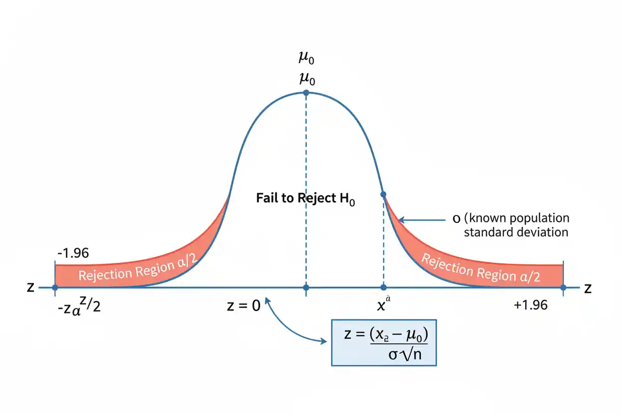

The one-sample z-test is an inferential statistical procedure used to evaluate whether a population mean differs from a specified reference value when the population standard deviation is known and the sampling conditions justify a normal reference distribution. It compares the observed sample mean with the mean stated by the null hypothesis and expresses their difference in units of the sample mean’s standard error. The resulting z statistic indicates how many standard errors the observed sample mean lies above or below the hypothesized population mean. Because the relevant population standard deviation σ is treated as known, the standardized statistic is evaluated using the standard normal distribution rather than Student’s t distribution.
The procedure may be two-sided when departures in either direction matter or one-sided when the research question specifies a direction in advance. A sufficiently extreme z statistic provides evidence against the null hypothesis, but statistical significance does not establish that the difference is practically important. The familiar idea that a z-test should automatically replace a t-test whenever a sample becomes “large” is incorrect; the classical distinction depends primarily on whether σ is genuinely known rather than on an arbitrary sample-size cutoff. Reliable inference also requires an appropriate sampling design, sufficiently independent observations, and a sampling distribution of the mean that is normal or adequately approximated by normality.
The one-sample z-test belongs to Statistics & Probability and the broader Inference & Regression framework. Its purpose is narrowly focused on testing one population mean against a specified benchmark under known-σ conditions.
What Is a One-Sample Z-Test?
A one-sample z-test evaluates a claim about one unknown population mean μ using a sample mean x̄. The classical version assumes that the population standard deviation σ is known.
For a two-sided test, the hypotheses are commonly:
H₀: μ = μ₀
H₁: μ ≠ μ₀
where μ₀ is the reference mean specified by the Null Hypothesis.
The test statistic is:
z = (x̄ − μ₀) / (σ / √n)
where:
- x̄ = sample mean
- μ₀ = hypothesized population mean
- σ = known population standard deviation
- n = sample size
The numerator measures the observed difference from the null value. The denominator measures the standard deviation of the sample mean under the assumed sampling model.
The test therefore asks whether the observed mean is unusually far from μ₀ relative to the amount of sampling variability expected when H₀ is true.
One-Sample Z-Test Formula
The central formula is:
z = (x̄ − μ₀) / SE(x̄)
When σ is known:
SE(x̄) = σ / √n
Therefore:
z = (x̄ − μ₀) / (σ / √n)
A positive z statistic indicates:
x̄ > μ₀
A negative z statistic indicates:
x̄ < μ₀
The absolute magnitude tells how far the sample mean lies from the hypothesized population mean in standard-error units.
For example:
z = 2.5
means the observed sample mean lies 2.5 standard errors above μ₀.
Similarly:
z = −2.5
means it lies 2.5 standard errors below μ₀.
The sign communicates direction; the magnitude determines how extreme the observed result is under the null reference distribution.
Why the Standard Error Uses σ
The standard deviation σ describes variation among individual population observations. The sample mean is less variable because averaging multiple independent observations reduces random variation.
For independent observations:
SD(x̄) = σ / √n
When σ is known, this quantity is also the standard error used by the z-test:
SE(x̄) = σ / √n
Suppose:
σ = 20
and:
n = 100
Then:
SE(x̄) = 20 / √100
SE(x̄) = 20 / 10
SE(x̄) = 2
Individual observations vary on a scale of 20 units, while repeated sample means of size 100 vary on a scale of only 2 units around μ.
That reduction in variability is why sample means can estimate population means more precisely as sample size increases.
Worked Example: Two-Sided One-Sample Z-Test
Suppose a production process is specified to have a population mean of 100 units. Long-term process information establishes a population standard deviation of:
σ = 12
A random sample of:
n = 36
observations produces:
x̄ = 104
The question is whether the population mean differs from 100.
The hypotheses are:
H₀: μ = 100
H₁: μ ≠ 100
First calculate the standard error:
SE(x̄) = 12 / √36
SE(x̄) = 12 / 6
SE(x̄) = 2
Now calculate the z statistic:
z = (104 − 100) / 2
z = 4 / 2
z = 2
The observed sample mean lies two standard errors above the null value.
For a two-sided test at:
α = 0.05
the standard normal critical values are approximately:
−1.96 and +1.96
Because:
2 > 1.96
the observed z statistic falls inside the upper rejection region.
The null hypothesis is therefore rejected at the 5% significance level.
Interpreting the Example Correctly
The statistical conclusion is that the sample provides evidence that the population mean differs from 100 under the assumptions of the z-test.
It would be incorrect to say:
There is a 95% probability that μ is not 100.
The procedure does not assign a posterior probability to H₀.
It would also be inappropriate to say that the four-unit difference is automatically important simply because it crosses the statistical rejection threshold. Whether four units matter depends on the process tolerance, financial consequences, safety requirements, or other practical context.
The z-test evaluates statistical evidence about the benchmark. Practical importance requires a separate judgment about the magnitude of the difference.
Standard Normal Reference Distribution
Under H₀ and the assumptions of the classical one-sample z-test:
Z ∼ N(0, 1)
The standard normal distribution has:
mean = 0
and:
standard deviation = 1
The observed z statistic is compared against this reference distribution.
Values near zero indicate that x̄ lies relatively close to μ₀ compared with its standard error. Large positive or negative values indicate increasingly unusual sample means under H₀.
The standard normal distribution is symmetric, so:
P(Z > c) = P(Z < −c)
for corresponding positive and negative cutoffs.
This symmetry produces the familiar ± critical values used in two-sided z-tests.
Two-Sided One-Sample Z-Test
A two-sided test is used when deviations above and below μ₀ are both scientifically or practically relevant.
The hypotheses are:
H₀: μ = μ₀
H₁: μ ≠ μ₀
At significance level:
α = 0.05
the total rejection probability is divided equally between both tails:
α/2 = 0.025
The standard normal critical values are approximately:
zcritical = ±1.96
The decision rule is:
Reject H₀ if z < −1.96 or z > 1.96
Equivalently:
Reject H₀ if |z| > 1.96
A result inside those boundaries leads to failure to reject H₀ at the 5% level.
Right-Tailed One-Sample Z-Test
A right-tailed test is appropriate when the alternative hypothesis states that the population mean exceeds the benchmark.
The hypotheses may be written:
H₀: μ = μ₀
H₁: μ > μ₀
At:
α = 0.05
the entire rejection probability is placed in the upper tail.
The critical value is approximately:
zcritical = 1.645
The decision rule is:
Reject H₀ if z > 1.645
Suppose:
z = 1.80
Then:
1.80 > 1.645
so H₀ is rejected at the 5% significance level.
A right-tailed alternative should be justified before examining the sample rather than selected after discovering that x̄ happens to exceed μ₀.
Left-Tailed One-Sample Z-Test
A left-tailed test evaluates whether the population mean is below the reference value.
The hypotheses are:
H₀: μ = μ₀
H₁: μ < μ₀
At:
α = 0.05
the standard normal critical value is approximately:
zcritical = −1.645
The decision rule is:
Reject H₀ if z < −1.645
Suppose:
z = −2.10
Then:
−2.10 < −1.645
and H₀ is rejected.
The negative sign is not evidence of weaker statistical significance. It simply reflects the direction of the observed sample departure.
Worked Example: Right-Tailed Test
Suppose a machine is historically calibrated to produce an average output of:
μ₀ = 50
The known population standard deviation is:
σ = 10
A sample of:
n = 100
produces:
x̄ = 52
The research question asks whether the population mean has increased.
The hypotheses are:
H₀: μ = 50
H₁: μ > 50
The standard error is:
SE(x̄) = 10 / √100
SE(x̄) = 1
The test statistic is:
z = (52 − 50) / 1
z = 2
At α = 0.05 for a right-tailed test:
zcritical ≈ 1.645
Because:
2 > 1.645
H₀ is rejected.
The sample provides evidence that the population mean exceeds 50.
Worked Example: Nonsignificant Result
Suppose instead:
x̄ = 50.8
while:
μ₀ = 50
σ = 10
n = 100
The standard error remains:
SE(x̄) = 1
Therefore:
z = (50.8 − 50) / 1
z = 0.8
For a two-sided test at α = 0.05:
|0.8| < 1.96
so H₀ is not rejected.
The correct conclusion is that the sample does not provide sufficiently strong evidence that the population mean differs from 50.
It would be incorrect to conclude that:
μ = 50 has been proven.
The observed data remain subject to sampling uncertainty.
The P-Value
The P-Value measures how extreme the observed z statistic is under H₀ according to the specified test direction.
For a right-tailed test:
p-value = P(Z ≥ zobserved | H₀)
For a left-tailed test:
p-value = P(Z ≤ zobserved | H₀)
For a two-sided test with a symmetric standard normal distribution:
p-value = 2P(Z ≥ |zobserved| | H₀)
Suppose:
z = 2
For a two-sided test:
p ≈ 0.0455
At:
α = 0.05
we have:
p < α
so H₀ is rejected.
The p-value is not:
P(H₀ is true | data)
That interpretation reverses the conditioning and is incorrect in the conventional frequentist framework.
P-Value and Critical-Value Methods Agree
Suppose a two-sided z-test uses:
α = 0.05
The critical values are:
±1.96
If:
z = 2.20
the critical-value method rejects H₀ because:
|2.20| > 1.96
The two-sided p-value is also below 0.05, so the p-value method reaches the same conclusion.
Likewise, if:
z = 1.20
then:
|1.20| < 1.96
and:
p > 0.05
Both approaches fail to reject H₀.
These are two representations of the same inferential decision when the same test assumptions and significance level are used.
Common Standard Normal Critical Values
Frequently used z critical values include:
| Significance Level | Test Structure | Critical Value |
|---|---|---|
| α = 0.10 | Two-sided | ±1.645 |
| α = 0.05 | Two-sided | ±1.960 |
| α = 0.01 | Two-sided | ±2.576 |
| α = 0.10 | One-sided | ±1.282 |
| α = 0.05 | One-sided | ±1.645 |
| α = 0.01 | One-sided | ±2.326 |
For one-sided tests, the sign depends on whether the rejection region is in the lower or upper tail.
These cutoffs are properties of the standard normal distribution. They do not automatically apply to t, chi-square, F, or other reference distributions.
Confidence Interval Connection
The same known-σ framework can produce a confidence interval for μ.
A normal-based confidence interval has the form:
x̄ ± z* × σ / √n
For a 95% confidence interval:
z* ≈ 1.96
Return to the example:
x̄ = 104
σ = 12
n = 36
The standard error is:
SE(x̄) = 2
The margin of error is:
1.96 × 2 = 3.92
Therefore:
Lower bound = 104 − 3.92 = 100.08
Upper bound = 104 + 3.92 = 107.92
The 95% confidence interval is:
100.08 to 107.92
The null value:
μ₀ = 100
lies just outside the interval, which corresponds to rejecting H₀: μ = 100 in the matching two-sided α = 0.05 z-test.
What the Confidence Interval Means
A frequentist 95% confidence interval does not mean:
There is a 95% probability that μ lies between 100.08 and 107.92.
Once the sample has been observed, μ is treated as a fixed parameter in the conventional frequentist framework.
The 95% refers to the interval-producing method: if the sampling procedure were repeated many times and a confidence interval constructed each time according to the same method, approximately 95% of those intervals would contain the true μ under the model assumptions.
The interval is still extremely useful because it communicates both the estimated location of μ and the precision of that estimate.
One-Sample Z-Test vs One-Sample T-Test
The One-Sample T-Test and one-sample z-test examine similar hypotheses about a population mean, but the classical versions differ in how population variability is handled.
For the z-test:
z = (x̄ − μ₀) / (σ / √n)
where:
σ is known
For the t-test:
t = (x̄ − μ₀) / (s / √n)
where:
σ is unknown and s estimates it
The t distribution has heavier tails because estimating σ introduces additional uncertainty.
As the t-test’s degrees of freedom become large, its reference distribution approaches the standard normal distribution, making numerical results increasingly similar.
However, similarity at large n does not eliminate the conceptual distinction between known σ and estimated σ.
Large Sample Does Not Automatically Mean Z-Test
A frequently repeated rule says:
n ≥ 30 → use z-test
and:
n < 30 → use t-test
This is not an accurate general rule for testing a population mean.
If σ is unknown, as it usually is in real applications, the standard t procedure remains appropriate even when:
n = 100
n = 1,000
or larger.
With large df, the t distribution becomes nearly indistinguishable from the standard normal distribution, so the numerical difference may be tiny. That does not mean the population standard deviation suddenly became known.
The test should follow the statistical information available rather than an arbitrary sample-size threshold.
When Is σ Truly Known?
The known-σ assumption deserves careful attention because it is uncommon for a population standard deviation to be known exactly.
It may be reasonable when the process has a well-established population variance based on stable historical measurement, a physical system has a genuinely known error distribution, or the analysis is a theoretical exercise in which σ is specified.
Using a standard deviation estimated from the same sample and simply labeling it σ does not create a genuine z-test.
If the quantity in the denominator is:
s
calculated from the current sample as an estimate of an unknown σ, the classical t framework is generally the relevant one for mean inference.
Normal Population Case
If the population observations are normally distributed and σ is known, then the sample mean is exactly normal for any positive sample size under independent sampling:
x̄ ∼ N(μ, σ²/n)
Therefore, under H₀:
Z = (x̄ − μ₀) / (σ / √n)
follows the standard normal distribution exactly.
A large sample is not required for this exact normal-population result.
This is an important distinction: sample size becomes particularly relevant when normality of the sample mean is being justified through an approximation rather than inherited exactly from a normal population.
Non-Normal Populations
The underlying population does not always need to be perfectly normal for a z-based approximation to become useful.
Under appropriate independence and finite-variance conditions, the sampling distribution of x̄ can approach normality as n increases. This is the central reasoning behind many large-sample approximations.
However, the convergence rate depends on the population distribution.
A mildly skewed, light-tailed population may produce a good approximation relatively quickly. A highly skewed or heavy-tailed population may require a much larger sample.
There is therefore no universal sample size at which every population produces an adequately normal sampling distribution.
Why There Is No Universal n = 30 Rule
The number 30 is sometimes used as a classroom heuristic for approximate normality of the sample mean, but it is not a universal mathematical threshold.
Consider two populations.
Population A is symmetric and light-tailed. Its sample mean may be approximately normal even with fewer than 30 observations.
Population B is extremely right-skewed and occasionally produces values hundreds of times larger than its typical observations. Its sampling distribution may remain noticeably skewed even at sample sizes far above 30.
Approximation quality depends on the underlying population’s skewness, tail behavior, outliers, and the precision required by the application.
Sample size should therefore be interpreted together with distributional behavior.
Independence of Observations
The standard-error formula:
σ / √n
assumes an appropriate independence structure.
If observations are positively correlated, the true sampling variability of x̄ can be larger than the ordinary formula suggests.
Examples include:
- repeated measurements on the same person
- employees within the same team
- students within the same classroom
- neighboring time-series observations
- geographically clustered measurements
Treating correlated observations as independent can make the standard error too small and the z statistic artificially large.
A large nominal n does not compensate for dependence. The analytical procedure must reflect the actual sampling structure.
Random Sampling and Representation
A mathematically correct z statistic cannot guarantee that a sample represents the target population.
Suppose an online survey collects thousands of voluntary responses. Even with:
n = 100,000
selection bias may prevent those respondents from representing the broader population.
A very small standard error only quantifies sampling uncertainty under the statistical sampling model. It does not account automatically for systematic bias arising from nonresponse, convenience sampling, measurement error, or other design problems.
Statistical precision and representativeness are separate properties.
Standard Deviation vs Standard Error
The population standard deviation:
σ
describes variability among individual observations.
The standard error:
σ / √n
describes variability of the sample mean across repeated samples.
Suppose:
σ = 30
and:
n = 225
Then:
SE(x̄) = 30 / √225
SE(x̄) = 30 / 15
SE(x̄) = 2
Individual observations vary on a scale of 30 units, but sample means based on 225 observations vary on a scale of only 2 units.
Confusing σ with the standard error can produce severely incorrect test statistics.
Effect of Increasing Sample Size
The standard error decreases according to:
SE(x̄) = σ / √n
If n increases from 25 to 100 while σ remains constant, sample size increases by a factor of four.
The standard error changes from:
σ / 5
to:
σ / 10
so it is cut in half.
As the standard error decreases, a fixed raw difference:
x̄ − μ₀
corresponds to a larger absolute z statistic.
This makes smaller departures from H₀ statistically detectable in large samples.
It does not make the underlying effect larger.
Statistical Significance vs Practical Significance
Suppose:
μ₀ = 100
A huge sample produces:
x̄ = 100.1
If the standard error is:
0.01
then:
z = (100.1 − 100) / 0.01
z = 10
The result is extremely statistically significant, yet the estimated difference is only:
0.1 unit
Whether 0.1 matters depends entirely on the application.
A statistical test therefore answers whether the difference is distinguishable from the null benchmark at the available precision. It does not determine whether that difference is valuable, harmful, clinically meaningful, economically significant, or operationally important.
Effect Size and the Z Statistic
The z statistic should not be interpreted as the size of the effect in original units.
Suppose:
z = 3
This means the observed sample mean lies three standard errors from μ₀.
It does not mean:
x̄ − μ₀ = 3 units
A standardized difference relative to the population standard deviation could instead be written:
d = (x̄ − μ₀) / σ
For the one-sample known-σ setting:
z = d√n
This relationship illustrates why the z statistic increases with sample size even when the standardized population-scale difference remains the same.
Inferential evidence and effect magnitude are related but distinct.
Type I Error
A Type I error occurs when the test rejects H₀ even though H₀ is true.
At:
α = 0.05
a correctly calibrated test is designed so that:
P(reject H₀ | H₀ true) = 0.05
under the test assumptions.
For a two-sided standard normal test, this probability is divided between the two rejection tails.
Type I error control is one reason the critical boundaries are defined before observing the result.
It does not mean that after rejecting H₀ there is automatically a 5% probability the conclusion is wrong.
Type II Error and Statistical Power
A Type II error occurs when the procedure fails to reject H₀ even though a relevant alternative is true.
Statistical power is the probability of correctly rejecting H₀ under a specified alternative:
Power = 1 − β
Power generally increases when:
- the true difference from μ₀ becomes larger
- n becomes larger
- σ becomes smaller
- α becomes less restrictive
- observations provide more independent information
A nonsignificant result in a low-powered study therefore provides limited evidence that the population mean is exactly equal to μ₀.
Failure to Reject Is Not Proof of Equality
Suppose:
H₀: μ = 50
and a test produces:
z = 0.40
with:
p > 0.05
The correct conclusion is:
Fail to reject H₀.
It is not:
Accept H₀ as proven.
The sample may simply be compatible with a range of possible population means around 50.
If the research objective is to demonstrate that μ is sufficiently close to 50 for practical purposes, an equivalence framework with a prespecified acceptable margin is more appropriate than using nonsignificance as proof of equality.
One-Sample Z-Test and Multiple Regression
The one-sample z-test evaluates one population mean against one specified benchmark. Multiple Regression addresses a different problem: modeling a quantitative response as a function of several predictors simultaneously.
Both methods can involve standardized statistics and normal approximations in particular inferential settings, but they should not be treated as interchangeable.
A one-sample z-test does not adjust a mean comparison for multiple predictors, estimate conditional slopes, or model interactions.
Its statistical question is intentionally narrow:
Is one population mean compatible with μ₀ under the known-σ sampling model?
Keeping that scope clear prevents a basic mean test from being expanded into a general regression procedure.
One-Sample Z-Test vs One-Way ANOVA
A one-sample z-test compares one population mean with one fixed benchmark. One-Way ANOVA is designed for evaluating equality among several group means under its own assumptions and F-based framework.
For example, testing:
H₀: μ = 100
is a one-sample problem.
Testing whether:
μ₁ = μ₂ = μ₃ = μ₄
is a multi-group problem.
Performing a sequence of one-sample z-tests does not reproduce the structure or error control of a properly specified ANOVA problem.
The number and relationship of the populations being compared should determine the inferential method.
One-Sample Mean Z-Test vs Proportion Z Procedures
The term z-test is also used for statistical procedures involving proportions because suitably standardized proportions can have approximately standard normal sampling distributions.
However, the formulas differ.
For the one-sample mean z-test discussed here:
z = (x̄ − μ₀) / (σ / √n)
A one-sample proportion test instead uses a standard error derived from the null proportion.
These procedures share a standard normal reference distribution but test different population parameters.
Using the correct formula requires identifying whether the target parameter is a mean, proportion, difference, regression coefficient, or another quantity before performing the test.
When to Use a One-Sample Z-Test
The classical mean z-test is appropriate when the research question concerns one population mean and:
- the reference value μ₀ is clearly specified
- the population standard deviation σ is genuinely known
- observations provide appropriately independent information
- the sampling design supports inference to the target population
- the sample mean is normally distributed or adequately approximated by normality
When σ must be estimated from the same sample, the One-Sample T-Test is generally the more appropriate classical procedure.
The decision should follow these statistical conditions rather than a rigid sample-size rule.
When Not to Use the Test
The ordinary one-sample z-test is not appropriate merely because software can calculate a z statistic.
Do not use the classical known-σ formula when σ is actually unknown and replaced by the current sample’s standard deviation without acknowledging that estimation.
The test is also unsuitable when observations are strongly dependent but treated as independent, when the outcome is not meaningfully quantitative for a mean comparison, or when severe selection bias makes population inference unsupported.
Extreme heavy tails or influential observations may also make the sample mean and normal approximation unreliable at the available sample size.
The statistical method should reflect the estimand, sampling design, and data-generating process.
Common Mistakes
A common mistake is believing that every sample with more than 30 observations requires a z-test. The classical distinction from the t-test depends primarily on whether σ is known.
Another error is using the sample standard deviation s in:
z = (x̄ − μ₀) / (s / √n)
and calling the result an exact classical z-test. Once σ is estimated from the sample, Student’s t framework accounts for that additional uncertainty.
A third mistake is interpreting the p-value as the probability that H₀ is true. It is calculated assuming H₀.
Researchers also sometimes interpret statistical significance as proof of practical importance. A tiny difference can produce a very large z statistic when n is enormous.
Another error is ignoring dependence because the dataset contains many rows. Correlated observations may provide substantially less independent information than their row count suggests.
Finally, failure to reject H₀ does not establish exact equality.
How to Perform a One-Sample Z-Test
Begin by defining the population mean and null benchmark:
H₀: μ = μ₀
Specify the alternative based on the research question:
Two-sided:
H₁: μ ≠ μ₀
Right-sided:
H₁: μ > μ₀
Left-sided:
H₁: μ < μ₀
Verify that the relevant population standard deviation σ is known and that the sampling assumptions are appropriate.
Calculate the sample mean:
x̄ = Σxᵢ / n
Then calculate the standard error:
SE(x̄) = σ / √n
Calculate the z statistic:
z = (x̄ − μ₀) / (σ / √n)
Finally, obtain the corresponding p-value or compare z with the appropriate standard normal critical value and interpret the result in the context of the original population mean question.
How to Report a One-Sample Z-Test
A useful result should communicate both the inferential decision and the actual observed difference.
Suppose:
μ₀ = 100
x̄ = 104
σ = 12
n = 36
and:
z = 2.00
A concise result could state that the sample mean was four units above the hypothesized population mean and that the two-sided z-test provided evidence against H₀ at the 5% level:
z = 2.00, p ≈ 0.0455
A stronger report would also include a confidence interval and explain whether a four-unit difference is practically meaningful.
Reporting only “significant” removes much of the information readers need.
Frequently Asked Questions
What is a one-sample z-test?
A one-sample z-test evaluates whether one population mean differs from a specified reference value when the population standard deviation is known and the normal-reference conditions are appropriate.
What is the one-sample z-test formula?
The classical formula is:
z = (x̄ − μ₀) / (σ / √n)
What does x̄ mean?
x̄ is the sample mean calculated from the observed data.
What does μ₀ mean?
μ₀ is the population mean specified under the null hypothesis.
What does σ mean?
σ is the known population standard deviation.
What is the standard error?
For the classical one-sample mean z-test:
SE(x̄) = σ / √n
What does the z statistic tell you?
It tells how many standard errors the observed sample mean lies above or below the hypothesized population mean.
What is the null hypothesis?
A common null is:
H₀: μ = μ₀
Can a one-sample z-test be two-sided?
Yes. A two-sided alternative is:
H₁: μ ≠ μ₀
Can it be one-sided?
Yes. Directional alternatives can be:
H₁: μ > μ₀
or:
H₁: μ < μ₀
when justified by the research question.
What is the critical value for a two-sided 5% z-test?
Approximately:
±1.96
What is the critical value for a one-sided 5% z-test?
Approximately:
+1.645
for an upper-tail test, or:
−1.645
for a lower-tail test.
What is the difference between a z-test and t-test?
The classical one-sample z-test uses known population standard deviation σ. The one-sample t-test estimates unknown σ using sample standard deviation s and uses Student’s t reference distribution.
Should I use a z-test whenever n is greater than 30?
No. There is no universal n = 30 rule that determines whether a mean test should use z or t. Whether σ is known is central to the classical distinction.
Can a z-test be used with a small sample?
Yes, if the population is normal, σ is known, observations are appropriately independent, and the other conditions are satisfied. Large n is not inherently required in that exact setting.
Does the population have to be normal?
Not always. The sampling distribution of the mean can be approximately normal for non-normal populations when sample size and distributional conditions support the approximation. Convergence speed varies across populations.
Does a small p-value mean H₀ is probably false?
Not in the frequentist interpretation. The p-value is a probability calculated under the assumption that H₀ is true.
Does statistical significance mean the difference is important?
No. Statistical significance and practical importance are separate. The raw or standardized magnitude should be interpreted in context.
Does failing to reject H₀ prove the population mean equals μ₀?
No. It means the sample did not provide sufficiently strong evidence against μ₀ under the chosen test and threshold.
What happens as sample size increases?
The standard error decreases according to:
σ / √n
so smaller departures from μ₀ become easier to detect statistically when other conditions remain unchanged.
Key Takeaway
The one-sample z-test evaluates whether one population mean is consistent with a specified reference value when the population standard deviation is known. Its central statistic is:
z = (x̄ − μ₀) / (σ / √n)
with:
SE(x̄) = σ / √n
The statistic expresses the difference between the sample mean and null mean in standard-error units. Under H₀ and the required conditions, it is evaluated using the standard normal distribution.
For a two-sided test at α = 0.05, the familiar rejection boundaries are approximately:
z = −1.96 and z = +1.96
but the correct critical value depends on the test direction and significance level. The procedure should not be selected merely because a sample contains more than 30 observations; if σ is unknown and estimated using s, the classical one-sample t-test is generally the appropriate framework. Most importantly, a statistically significant z result provides evidence against the specified null mean but does not establish practical importance, while a nonsignificant result does not prove that the population mean exactly equals the benchmark.



