
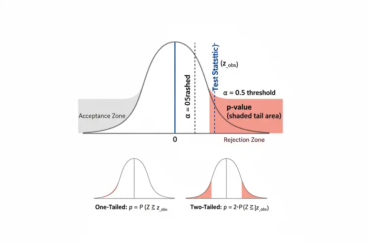

A p-value is a probability calculated under a specified null hypothesis that measures how extreme the observed test result is relative to what the null model predicts. More precisely, it is the probability—assuming the null hypothesis and the statistical model are correct—of obtaining a test statistic at least as incompatible with the null hypothesis as the statistic actually observed, where “at least as extreme” is defined by the particular statistical test. A small p-value indicates that the observed result lies in a relatively unusual part of the null distribution, while a large p-value indicates that the result is not especially unusual under that model.
The p-value does not state the probability that the null hypothesis is true, the probability that the alternative hypothesis is true, the probability that the result occurred “by chance,” or the size of the underlying effect. It is also strongly affected by sample size and precision, which means a very small effect can produce a very small p-value in a sufficiently large dataset. Statistical significance therefore should not be confused with practical importance. Correct interpretation requires understanding the null hypothesis, test statistic, reference distribution, test direction, significance level, study design, and assumptions that generated the p-value.
The p-value is one of the most widely used quantities in Statistics & Probability and appears throughout Inference & Regression. Its role is specific: it measures the extremeness of an observed test statistic under a null model rather than directly measuring effect magnitude, model quality, or the truth of a hypothesis.
What Is a P-Value?
A p-value is calculated after a test statistic has been obtained from sample data. Suppose a statistical test produces a statistic T and the null hypothesis determines the distribution of T when H₀ is true.
For an upper-tailed test, the p-value has the conceptual form:
p-value = P(T ≥ Tobserved | H₀)
For a lower-tailed test:
p-value = P(T ≤ Tobserved | H₀)
For a symmetric two-sided test, a common form is:
p-value = P(|T| ≥ |Tobserved| | H₀)
The exact calculation depends on the test statistic and its null distribution.
The vertical bar means “conditional on.” Therefore:
P(data this extreme | H₀)
is fundamentally different from:
P(H₀ | data)
The first is the type of probability used in a conventional p-value. The second is a probability about the hypothesis after observing the data and is not what a frequentist p-value provides.
The Core Meaning of a P-Value
Suppose a hypothesis test produces:
p = 0.03
A useful interpretation is:
If H₀ and the statistical model were correct, results at least as extreme as the observed result would occur with probability 0.03 according to this test.
This means the observed statistic lies in a relatively unusual region of its null reference distribution.
It does not mean:
There is a 3% probability that H₀ is true.
It also does not mean:
There is a 97% probability that H₁ is true.
Those statements assign probabilities directly to hypotheses, which the conventional p-value does not do.
The p-value evaluates data relative to a hypothesis. It does not reverse that relationship to evaluate the probability of the hypothesis given the data.
P-Value Formula
There is no single numerical formula that calculates every p-value because different statistical tests use different reference distributions. The general structure is:
p-value = null-distribution probability of results at least as extreme as the observed test statistic
For an upper-tail statistic:
p = 1 − F(Tobserved)
where F is the cumulative distribution function of T under H₀.
For a lower-tail statistic:
p = F(Tobserved)
For a symmetric two-sided test with a positive observed statistic:
p = 2[1 − F(|Tobserved|)]
when that doubling rule is appropriate for the test.
The p-value therefore depends on two ingredients:
the observed test statistic
and:
its distribution under H₀
A raw sample difference alone is not enough to determine a p-value.
Worked Example Using a Z Statistic
Suppose a test of a population mean produces:
z = 2.00
and the alternative hypothesis is two-sided.
Under H₀:
Z ∼ N(0, 1)
The upper-tail probability beyond z = 2 is approximately:
P(Z ≥ 2) ≈ 0.0228
Because the test is two-sided and the standard normal distribution is symmetric:
p ≈ 2 × 0.0228
p ≈ 0.0456
Thus:
p ≈ 0.0455
after ordinary rounding.
If the significance level is:
α = 0.05
then:
p < α
so H₀ is rejected at the 5% significance level.
The same underlying known-σ mean-testing framework is developed in the One-Sample Z-Test.
What Does p = 0.0455 Mean?
For the preceding two-sided z-test, p ≈ 0.0455 means that if H₀ and the model were correct, the probability of obtaining a z statistic with magnitude at least as large as 2.00 would be approximately 4.55%.
Symbolically:
P(|Z| ≥ 2.00 | H₀) ≈ 0.0455
The probability includes both tails because the alternative treats sufficiently large departures in either direction as evidence against H₀.
It would be incorrect to say:
H₀ has a 4.55% probability of being true.
The p-value is computed under the assumption of H₀ rather than being a probability assigned to H₀.
One-Sided P-Values
Consider the same observed statistic:
z = 2.00
Suppose the research question specifies a right-tailed alternative in advance.
The p-value is now:
p = P(Z ≥ 2.00)
p ≈ 0.0228
The two-sided p-value was approximately 0.0455, while the right-sided value is approximately 0.0228.
This difference occurs because the two-sided procedure counts extreme results in both directions, while the right-sided procedure counts only the upper tail.
A one-sided p-value should not be selected simply because the observed statistic happens to point in the preferred direction. The test direction should follow the research question established independently of the observed result.
Left-Sided P-Values
Suppose:
z = −2.00
and the alternative is:
H₁: parameter < null value
The p-value is:
p = P(Z ≤ −2.00)
p ≈ 0.0228
If the alternative were instead right-sided, this negative statistic would not provide evidence in the hypothesized direction, and the one-sided p-value would be large.
This illustrates why the sign of a test statistic matters in directional testing.
The p-value is not determined solely by absolute magnitude; it also depends on how extremeness is defined by the alternative hypothesis.
Two-Sided P-Values
A two-sided test treats sufficiently large departures on either side of the null value as evidence against H₀.
For a symmetric statistic such as the standard normal z statistic, a common formula is:
p = 2P(Z ≥ |zobserved|)
Suppose:
zobserved = −2.50
Then:
|zobserved| = 2.50
The one-tail probability beyond 2.50 is approximately:
0.0062
Therefore:
p ≈ 2 × 0.0062
p ≈ 0.0124
The negative sign identifies the direction of the sample departure, but the two-sided p-value measures extremeness in either direction.
For asymmetric or discrete test statistics, two-sided p-value definitions can require more care than simply doubling one tail.
The P-Value and Significance Level
The significance level α is a threshold selected for the statistical testing procedure, commonly before interpreting the observed result.
Frequently encountered values include:
α = 0.10
α = 0.05
α = 0.01
The usual decision rule is:
If p ≤ α, reject H₀.
If p > α, fail to reject H₀.
Suppose:
p = 0.032
and:
α = 0.05
Then:
0.032 < 0.05
so H₀ is rejected.
If instead:
α = 0.01
then:
0.032 > 0.01
so H₀ is not rejected at the 1% level.
The p-value has not changed. Only the decision threshold has changed.
P-Value vs Alpha
The p-value and α should not be treated as interchangeable.
The p-value is calculated from the observed sample and the null reference distribution.
The significance level is a decision threshold chosen for the testing procedure.
Conceptually:
p-value = property of the observed test result under H₀
while:
α = prespecified rejection threshold
A result such as:
p = 0.049
crosses:
α = 0.05
but does not cross:
α = 0.01
There is no meaningful transformation by which p = 0.049 suddenly becomes qualitatively strong evidence while p = 0.051 becomes no evidence at all. The numerical p-value should be considered alongside the effect estimate, uncertainty, design, and context.
P-Value and Critical-Value Approaches
A hypothesis test can often be performed either by calculating a p-value or by comparing the test statistic with a critical value.
Suppose a two-sided standard normal test uses:
α = 0.05
The critical boundaries are approximately:
−1.96 and +1.96
If:
z = 2.30
then:
|2.30| > 1.96
so H₀ is rejected.
The associated two-sided p-value is approximately:
p ≈ 0.021
which also satisfies:
p < 0.05
The two approaches therefore produce the same decision when the same test, significance level, and assumptions are used.
The p-value has the advantage of showing the tail probability associated with the observed statistic rather than only whether one predefined threshold was crossed.
Worked Example With a One-Sample T-Test
Suppose a sample gives:
n = 25
x̄ = 53
s = 5
and the null hypothesis states:
H₀: μ = 50
The estimated standard error is:
SE(x̄) = 5 / √25
SE(x̄) = 1
The test statistic is:
t = (53 − 50) / 1
t = 3
The degrees of freedom are:
df = 25 − 1
df = 24
For a two-sided test:
p ≈ 0.006
This p-value means that under H₀ and the t-model assumptions, a t statistic with magnitude at least 3 would be relatively unusual.
The underlying procedure and its assumptions are discussed in the One-Sample T-Test.
P-Values Depend on the Reference Distribution
The same numerical test statistic can produce different p-values under different reference distributions.
For example:
statistic = 2
does not uniquely determine a p-value.
If the statistic is standard normal and the test is two-sided:
p ≈ 0.0455
If it is a t statistic with very few degrees of freedom, the heavier tails of the t distribution produce a larger two-sided p-value.
If it is an F statistic, only an upper-tail probability may be relevant and the reference distribution is completely different.
Therefore, a reported p-value should always be understood in the context of the statistical test from which it came.
P-Values in One-Way ANOVA
A One-Way ANOVA uses an F statistic to evaluate whether several independent population means are all equal.
The p-value takes the upper-tail form:
p = P(Fdf₁,df₂ ≥ Fobserved | H₀)
Suppose:
Fobserved = 6.5
The p-value is determined by the F distribution with the appropriate numerator and denominator degrees of freedom.
A small p-value provides evidence against:
H₀: μ₁ = μ₂ = … = μₖ
It does not identify which specific groups differ. That requires additional analysis.
This illustrates an important general principle: a p-value inherits its meaning from the null hypothesis and test statistic that generated it.
P-Values in Paired Data
A Paired T-Test usually reduces paired observations to within-pair differences and tests whether the population mean difference equals a specified value, commonly zero.
If D represents the paired difference, a standard null is:
H₀: μD = 0
The t statistic is based on:
D̄
relative to the standard error of the mean difference.
The resulting p-value measures how extreme that paired-difference statistic is under the null model.
Treating paired measurements as though they were independent changes the standard error structure and can therefore change the p-value substantially.
A p-value is only as valid as the model and sampling structure used to calculate it.
A Small P-Value Is Not the Probability H₀ Is True
This is the most important interpretation error to avoid.
Suppose:
p = 0.01
The p-value represents:
P(data at least this extreme | H₀)
It does not represent:
P(H₀ | data)
These probabilities are conceptually different.
A simple analogy illustrates the distinction. The probability of observing smoke given that there is a fire can be high, but the probability of fire given smoke depends on other possible causes of smoke and prior information. Reversing the conditioning changes the question.
Likewise, converting a p-value into a probability that H₀ is true requires additional assumptions and a different inferential framework.
A P-Value Is Not the Probability the Result Is Due to Chance
Statements such as:
“There is only a 2% chance the result happened by chance.”
are generally misleading.
Random sampling variation is already part of the statistical model. The p-value does not divide the world into “chance” and “not chance” and then assign probabilities to those explanations.
Instead, it asks how often results at least as extreme would occur under a specific null model that includes random variability.
A result can have a small p-value and still be affected by bias, measurement error, confounding, model misspecification, selective reporting, or other non-random problems.
The p-value only addresses the probability calculation implied by the specified statistical model.
A Large P-Value Does Not Prove H₀
Suppose:
p = 0.70
This means the observed test statistic is not unusual under H₀ according to the test.
It does not mean:
There is a 70% probability H₀ is true.
Nor does it prove the population parameter equals the null value.
A large p-value can arise when the null is approximately correct, but it can also occur when:
- sample size is small
- variability is high
- statistical power is low
- the effect is modest
- measurements are imprecise
Failing to reject H₀ should therefore not be described as demonstrating equality.
p = 0.05 Is Not a Natural Scientific Boundary
The value:
0.05
is a conventional threshold in many settings, not a fundamental law separating truth from falsehood.
Suppose two otherwise identical analyses produce:
p = 0.049
and:
p = 0.051
The statistical evidence represented by these values is extremely similar.
It is misleading to describe the first as a definitive discovery and the second as evidence of no effect merely because they lie on opposite sides of 0.05.
Threshold-based decisions may be necessary in some applications, but interpretation should preserve the underlying continuous evidence and uncertainty.
Smaller P-Values and Stronger Incompatibility
Within the same statistical model, a smaller p-value generally indicates greater incompatibility between the observed statistic and the null hypothesis according to that test.
For example:
p = 0.001
corresponds to a more extreme null-distribution position than:
p = 0.04
However, this does not mean the first study has a larger underlying effect.
A large sample can make a tiny effect produce p = 0.001, while a small sample can make a much larger observed effect produce p = 0.04.
The p-value therefore describes statistical evidence relative to the null model, not substantive magnitude.
Sample Size and the P-Value
Sample size can strongly influence a p-value because larger samples generally reduce standard errors.
Consider a mean difference:
x̄ − μ₀ = 1
If:
SE = 2
then:
statistic = 1 / 2 = 0.5
The p-value will be relatively large.
If the same one-unit effect is estimated with:
SE = 0.1
then:
statistic = 1 / 0.1 = 10
and the p-value will be extremely small.
The effect magnitude has not changed. The precision has.
This is why statistical significance becomes easier to achieve as the amount of independent information increases.
Statistical Significance vs Practical Importance
Suppose a website experiment estimates an improvement of:
0.05 percentage points
With tens of millions of observations, the p-value could be extremely small.
The statistical conclusion may be that the null hypothesis of exactly zero difference is incompatible with the data.
Whether a 0.05-percentage-point improvement matters commercially is an entirely different question.
Conversely, a small experiment may estimate a large improvement but produce a p-value above 0.05 because uncertainty is substantial.
The p-value should therefore be interpreted alongside the actual effect estimate and its practical consequences.
P-Value vs Effect Size
An effect size quantifies how large a difference or relationship is. A p-value quantifies the extremeness of a test statistic under H₀.
Suppose Study A finds:
effect size = 0.10
p = 0.001
Study B finds:
effect size = 0.70
p = 0.08
Study A has stronger statistical evidence against its null model, while Study B has the larger point estimate of magnitude.
Neither pair of numbers should be interpreted in isolation.
This distinction is especially important in large datasets where tiny effects can be estimated very precisely.
P-Value and Confidence Intervals
For many standard two-sided tests, the p-value is closely related to whether a corresponding confidence interval contains the null value.
Suppose the null is:
H₀: μ = 50
If a compatible 95% confidence interval for μ is:
51.2 to 55.4
then 50 is excluded, which generally corresponds to:
p < 0.05
for the matching two-sided test.
If the interval is:
48.5 to 54.0
then 50 is included, which generally corresponds to:
p > 0.05
for the compatible procedure.
The confidence interval adds useful information because it displays a range of parameter values rather than only the tail probability relative to one null value.
P-Value vs Prediction Interval
A p-value and a Prediction Interval answer very different questions.
A p-value measures the extremeness of a test statistic under a null hypothesis.
A prediction interval provides a range intended to cover a future observation, under a specified predictive model and interval procedure.
For example, a regression coefficient may have a small p-value, indicating evidence that its population coefficient differs from zero, while prediction intervals around future observations remain wide because individual outcomes contain substantial unexplained variation.
Strong evidence about a parameter does not imply precise prediction of individual observations.
The inferential quantity should always be matched to the question being asked.
Exact and Approximate P-Values
Some p-values can be calculated exactly under a fully specified finite-sample distribution. Others use asymptotic approximations that become accurate as sample size grows under appropriate conditions.
For example, certain large-sample tests rely on:
test statistic ≈ reference distribution
rather than an exact equality of distributions.
An approximate p-value can be useful and highly accurate when its assumptions are satisfied, but it should not be treated as mathematically exact in every finite sample.
Approximation quality can deteriorate with sparse data, severe skewness, dependence, boundary parameters, or other irregular conditions.
The numerical precision displayed by software does not guarantee equivalent inferential precision.
Continuous vs Discrete Test Statistics
With continuous reference distributions, exact observed test-statistic values have probability zero, so p-values are naturally defined through tail areas.
With discrete data, however, the test statistic may take only a limited set of possible values. Tail probabilities can therefore jump rather than vary continuously.
As a result, discrete-test p-values may not be able to attain every numerical level such as exactly 0.05.
Different definitions of a two-sided p-value can also produce differences in some discrete testing problems.
The general principle remains the same: the p-value is determined by the null distribution and the definition of results considered at least as extreme.
Composite Null Hypotheses
Some null hypotheses contain more than one possible parameter value rather than a single exact point.
A one-sided problem might conceptually test:
H₀: μ ≤ μ₀
against:
H₁: μ > μ₀
The p-value is then calibrated so that its behavior appropriately controls error across the null parameter space, often using a boundary value that produces the most challenging null case.
This is more subtle than the simple statement:
“Assume μ = μ₀.”
The point-null examples are excellent foundations for learning p-values, but real statistical tests can involve broader null models and nuisance parameters.
Multiple Testing and P-Values
When many hypotheses are tested, interpreting every p-value using the same isolated 0.05 threshold can create a large number of false-positive findings.
Suppose 100 independent null hypotheses are all true and each is tested at:
α = 0.05
The expected number of false rejections is:
100 × 0.05 = 5
although the actual number will vary.
This does not mean every p-value must always be adjusted. The appropriate treatment depends on the inferential family and research objective.
It does mean that a p-value should not be interpreted without considering how many hypotheses were examined and how the testing plan was constructed.
Why Repeated Testing Can Be Misleading
Suppose a researcher repeatedly collects more observations, recomputes the same conventional p-value after every small batch, and stops as soon as:
p < 0.05
A standard fixed-sample test may no longer retain its nominal false-positive behavior under this unplanned stopping rule.
Similarly, repeatedly trying alternative variables, transformations, subgroup definitions, or model specifications until one produces a small p-value can make the reported value appear more surprising than the complete analysis process warrants.
A p-value’s calibration depends on the procedure that generated it, not merely the final equation shown in a report.
Selective Reporting
Imagine 20 outcomes are analyzed but only the one with:
p = 0.02
is reported.
Readers who see only that analysis may reasonably think one prespecified hypothesis produced p = 0.02. In reality, the result was selected from a much larger search.
This selective process changes the evidential context.
Transparent analysis requires readers to understand relevant multiplicity, exploratory choices, and selection procedures.
The p-value itself cannot reveal whether it was the only analysis performed or the smallest among hundreds.
P-Hacking and Data-Dependent Decisions
P-hacking refers broadly to analysis practices that increase the probability of obtaining conventionally significant p-values through data-dependent choices.
Examples can include:
- testing many outcomes without accounting for the search
- trying multiple exclusion rules
- switching between one-sided and two-sided tests after observing results
- repeatedly adding observations until significance appears
- testing many subgroup definitions
- reporting only favorable specifications
These practices do not necessarily involve fabricating data. The problem is that the nominal p-value no longer reflects the full process that produced the selected result.
Good statistical interpretation therefore requires transparency about analytical decisions.
P-Values and Model Assumptions
A p-value is calculated from a reference distribution whose validity depends on assumptions.
Potential assumptions can concern:
- independence
- distributional form
- variance structure
- sampling design
- model specification
- absence of severe influential observations
- correct handling of clustering or repeated measurements
If these assumptions are badly violated, the reported p-value may not have its intended interpretation.
For example, treating highly correlated observations as independent can make standard errors too small and p-values artificially low.
A p-value should therefore never be evaluated independently of the method that generated it.
Bias Is Not Fixed by a Small P-Value
Suppose a study contains a large systematic measurement error. Increasing the sample size may estimate the biased quantity with extraordinary precision, producing a very small p-value.
The result is statistically precise but still biased.
Likewise, confounding, nonresponse, convenience sampling, data leakage, and model misspecification do not disappear because:
p < 0.001
P-values quantify sampling-model extremeness, not the absence of systematic errors.
Study design and measurement quality can matter more than numerical significance.
P-Values Do Not Establish Causation
A small p-value for an association does not prove that one variable causes another.
Suppose an observational analysis finds:
p < 0.001
for an association between X and Y.
Possible explanations can include:
- X causes Y
- Y causes X
- a third variable affects both
- selection processes create the relationship
- measurement artifacts contribute
- the model is misspecified
The p-value addresses evidence against the tested null model. It does not identify the causal mechanism responsible for the observed association.
Causal inference requires suitable design and additional assumptions.
What Does p < 0.001 Mean?
When software reports:
p < 0.001
it means the calculated p-value is smaller than 0.001 at the displayed precision or reporting threshold.
This should not be rewritten as:
p = 0
A finite sample generally does not produce literal proof that the null model has zero probability.
Reporting:
p < 0.001
is often more appropriate than displaying an excessively long decimal such as:
p = 0.000000000034
when the extra digits add no useful interpretive information.
Extremely small p-values still do not measure effect magnitude.
Can a P-Value Equal 1?
Yes.
A p-value can equal or approach 1 when the observed statistic lies at a point of maximum compatibility with the null according to the test definition.
For example, in some symmetric two-sided tests, a test statistic of:
0
can produce:
p = 1
because the observed estimate equals the null value exactly and every possible statistic is at least as extreme according to the chosen distance measure.
This does not prove H₀. It simply means the observed test statistic provides no discrepancy from the null benchmark.
Can a P-Value Equal 0?
Software may display:
p = 0.000
because the true numerical value is smaller than the software’s display precision.
A mathematically calculated tail probability is generally better described as extremely small rather than exactly zero unless the test structure genuinely permits a zero probability.
Reporting:
p < 0.001
or another appropriate bound usually avoids the misleading suggestion of mathematical impossibility.
A tiny p-value indicates strong incompatibility with H₀ under the model, not absolute proof.
Does a Lower P-Value Mean a Larger Effect?
No.
Suppose Study A has:
estimated effect = 0.1
SE = 0.01
The standardized statistic is:
0.1 / 0.01 = 10
which gives an extremely small p-value.
Study B has:
estimated effect = 1.0
SE = 0.6
giving:
1.0 / 0.6 ≈ 1.67
and a much larger p-value.
Study B has the larger estimated effect, while Study A has the stronger evidence against zero because its estimate is far more precise.
P-values and effects must therefore be reported separately.
Does a Lower P-Value Mean a Better Study?
No.
A smaller p-value can result from:
- larger sample size
- lower variance
- larger effect
- different test assumptions
- model misspecification
- ignored dependence
- selective analysis
Study quality depends on design, measurement, sampling, transparency, assumptions, and relevance—not merely how many zeros appear after the decimal point.
A well-designed study with p = 0.08 can be more informative than a biased study with p < 0.0001.
How to Interpret a P-Value Correctly
Begin with the null hypothesis. Identify exactly what parameter value, relationship, or model condition is being tested.
Next identify the test statistic and its null distribution. Determine whether the test is one-sided or two-sided and whether the reference distribution is exact or approximate.
Then interpret the numerical p-value as a tail probability under H₀.
For example:
p = 0.02
means that results at least as extreme as the observed result would have probability 0.02 under the null model according to that test.
Only after this interpretation should the result be compared with α if a formal reject/fail-to-reject decision is required.
Finally, examine the effect estimate, confidence interval, study design, assumptions, and practical consequences.
How to Report a P-Value
A useful report should connect the p-value with the statistical test and observed effect rather than presenting it alone.
For example:
The sample mean was 3 units above the hypothesized value, t(24) = 3.00, p ≈ 0.006.
This provides:
- the observed effect
- the test statistic
- degrees of freedom
- p-value
If a confidence interval is available, including it provides additional information about precision.
Avoid reporting only:
p < 0.05
when the exact or reasonably rounded value is available and meaningful.
Also avoid describing results as merely “significant” or “not significant” without discussing magnitude.
Common P-Value Misconceptions
The most common mistake is:
p-value = probability H₀ is true
This is false.
Another common mistake is:
1 − p = probability H₁ is true
This is also false.
A third error is:
p-value = probability the result happened by chance
which misrepresents the conditional probability being calculated.
A fourth mistake is:
p > 0.05 proves no effect
which confuses insufficient evidence with evidence of exact equality.
A fifth error is:
smaller p-value means larger effect
which ignores the role of standard error and sample size.
Finally:
p < 0.05 proves causation
is incorrect because causal interpretation depends on design and assumptions rather than significance alone.
A Practical P-Value Checklist
Before interpreting a reported p-value, ask:
What exactly is H₀?
What statistic was tested?
Was the test one-sided or two-sided?
What reference distribution was used?
Were the relevant observations independent?
Were assumptions about variance, distribution, or model form reasonable?
Was the test prespecified or selected after inspecting the data?
Were many hypotheses tested?
What is the estimated effect size?
What is the confidence interval?
Is the effect practically important?
These questions place the p-value in its proper statistical context and prevent a single number from carrying more meaning than it actually contains.
Frequently Asked Questions
What is a p-value in simple terms?
A p-value measures how unusual the observed test result would be under the null hypothesis, counting results at least as extreme according to the statistical test.
What is the general p-value formula?
For an upper-tail test:
p = P(T ≥ Tobserved | H₀)
For a lower-tail test:
p = P(T ≤ Tobserved | H₀)
The exact formula depends on the reference distribution.
What does p = 0.05 mean?
It means results at least as extreme as the observed result have a 5% probability under H₀ according to the test. It does not mean H₀ has a 5% probability of being true.
What does p < 0.05 mean?
It means the calculated p-value lies below 0.05. If α was set at 0.05, the conventional decision is to reject H₀.
What does p > 0.05 mean?
It means the result does not cross an α = 0.05 rejection threshold. The correct conclusion is usually to fail to reject H₀, not to prove H₀ true.
Is a p-value the probability the null hypothesis is true?
No.
Is 1 − p the probability the alternative hypothesis is true?
No.
Does a small p-value prove causation?
No. It only provides evidence against a specified null model under the statistical assumptions.
Does a small p-value mean a large effect?
No. Large samples can produce extremely small p-values for tiny effects.
Can a large effect have a large p-value?
Yes. A large estimated effect can remain statistically uncertain when the sample is small or variability is high.
Is p = 0.049 fundamentally different from p = 0.051?
No. The evidential difference is tiny, even though a conventional α = 0.05 decision rule places them on opposite sides of a threshold.
Can a p-value be 1?
Yes, or very close to 1, when the observed statistic is highly compatible with the null model.
Can a p-value be zero?
Software may display zero because of rounding or numerical limits. Extremely small p-values should generally be reported using an appropriate inequality rather than interpreted as mathematical proof.
Why does sample size affect the p-value?
Larger samples usually reduce standard errors, making a given effect farther from the null value in standardized units.
What is the difference between p-value and alpha?
The p-value is calculated from the observed data under H₀. Alpha is a threshold chosen for the testing procedure.
What is the difference between a p-value and a confidence interval?
A p-value measures compatibility with one null hypothesis. A confidence interval provides a range of parameter values compatible with the data under the interval procedure and assumptions.
What is the difference between a p-value and a prediction interval?
A p-value evaluates a null hypothesis. A prediction interval provides a range for a future observation under a predictive model.
Should p-values be reported with effect sizes?
Usually yes. The p-value describes statistical evidence, while an effect estimate describes magnitude.
Does a nonsignificant p-value mean two groups are equivalent?
No. Demonstrating equivalence requires an analysis specifically designed around a meaningful equivalence margin.
Can multiple testing affect p-values?
The individual numerical p-values remain what they are, but interpreting many tests using isolated significance thresholds can greatly increase the overall false-positive risk.
Key Takeaway
A p-value is a conditional tail probability calculated under a null hypothesis. Its general meaning is:
p-value = P(result at least as extreme as observed | H₀)
For an upper-tailed test:
p = P(T ≥ Tobserved | H₀)
and for many symmetric two-sided tests:
p = P(|T| ≥ |Tobserved| | H₀)
A small p-value indicates that the observed test statistic is relatively unusual under the null model. It does not measure the probability that H₀ is true, the probability that H₁ is true, the probability that the result happened “by chance,” the size of the effect, or the practical importance of the finding.
The p-value also depends heavily on precision and sample size, so tiny effects can become highly statistically significant in large datasets. Reliable interpretation therefore requires more than comparing p with 0.05. The strongest analysis considers the null hypothesis, test statistic, reference distribution, test direction, effect magnitude, confidence interval, study design, assumptions, multiplicity, and real-world consequences together.



