Prediction Interval: Definition, Formula & Example

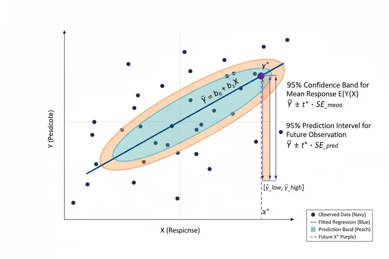
A prediction interval is a statistical interval designed to contain a future observation with a specified long-run coverage probability under a fitted model and its assumptions. Unlike a confidence interval for a population mean or regression mean response, a prediction interval must account for two sources of uncertainty: uncertainty in estimating the expected response and the natural variability of an individual future observation around that expected response. This additional variability makes a prediction interval wider than the corresponding confidence interval for the mean response at the same predictor value and confidence level. In simple linear regression, the interval expands as the predictor value moves farther from the center of the observed x-values because the fitted regression line becomes less precisely estimated there. It also reflects the residual standard deviation, so noisier data produce wider predictive ranges even when the fitted relationship is statistically clear.

A prediction interval is therefore fundamentally about forecasting an individual future outcome rather than estimating a fixed population parameter. Correct interpretation requires distinguishing prediction from parameter inference, recognizing that nominal coverage depends on the statistical model, and avoiding extrapolation far beyond the predictor values represented in the data.

Prediction intervals belong to Statistics & Probability and are an important part of Inference & Regression. They connect regression estimation with practical forecasting by expressing uncertainty around a future response rather than only around the fitted mean.

What Is a Prediction Interval?

Suppose a regression model predicts that a future observation will have:

ŷ₀ = 50

A point prediction of 50 does not imply the future outcome will equal exactly 50. Individual observations vary around the fitted regression relationship, and the estimated regression itself is also uncertain.

A prediction interval adds an uncertainty range around the point prediction.

For example:

Predicted value = 50

95% prediction interval = 38 to 62

The interpretation is not that there is automatically a 95% probability that one already-fixed future value lies between 38 and 62 in every philosophical framework. Under the conventional frequentist interpretation, the interval-producing procedure is designed so that, under repeated applications of the model and sampling process, approximately 95% of such prediction intervals contain their corresponding future observations when the assumptions hold.

This repeated-sampling coverage property is what defines the conventional prediction interval.

Prediction Interval vs Point Prediction

A point prediction gives a single estimated future value:

ŷ₀

A prediction interval gives a range:

Lower prediction limit to upper prediction limit

The point prediction is usually the center of a symmetric classical regression prediction interval:

ŷ₀ ± margin of prediction error

A point estimate alone hides uncertainty. Two models can both predict:

ŷ₀ = 50

while having very different predictive precision.

One model might produce:

48 to 52

while another produces:

20 to 80

The identical point prediction therefore does not imply equivalent predictive usefulness.

General Prediction Interval Structure

Many classical prediction intervals have the general form:

Point prediction ± critical value × prediction standard error

or:

ŷ₀ ± t* × SEprediction

The critical value reflects the desired coverage level and relevant reference distribution.

The prediction standard error incorporates uncertainty associated with estimating the expected response plus the variability of a future individual outcome.

This differs from a confidence interval for the conditional mean, whose standard error includes uncertainty about the estimated mean but not the full random deviation of a future observation.

Prediction Interval in Simple Linear Regression

Consider the population model:

Y = β₀ + β₁X + ε

A fitted sample regression is:

ŷ = b₀ + b₁x

where b₀ is the estimated Regression Intercept and b₁ is the estimated Regression Slope.

For a chosen predictor value x₀, the point prediction is:

ŷ₀ = b₀ + b₁x₀

A classical prediction interval for a new individual response at x₀ is:

ŷ₀ ± t* × sₑ × √[1 + 1/n + (x₀ − x̄)² / Σ(xᵢ − x̄)²]

where:

• ŷ₀ = predicted response at x₀
• t* = appropriate t critical value
• sₑ = residual standard error
• n = sample size
• x₀ = predictor value for the future observation
• x̄ = sample mean of the observed predictor values
• xᵢ = observed predictor values

The term under the square root determines how much predictive uncertainty applies at x₀.

The Most Important Term: The Extra 1

Compare the prediction interval standard-error factor:

√[1 + 1/n + (x₀ − x̄)² / Σ(xᵢ − x̄)²]

with the corresponding standard-error factor for a confidence interval for the mean response:

√[1/n + (x₀ − x̄)² / Σ(xᵢ − x̄)²]

The prediction interval contains an additional:

1

inside the square root.

That term represents the random variation of a new individual response around the true regression mean.

This is the fundamental mathematical reason the prediction interval is wider.

Even if the true regression line were estimated almost perfectly, individual future observations would still vary around that line because of residual variability.

Confidence Interval vs Prediction Interval

A confidence interval and prediction interval can be centered on the same fitted response but answer different questions.

A confidence interval for the mean response asks:

Where is the true average response at x₀ likely to be estimated by this procedure?

A prediction interval asks:

What range should cover a new individual response at x₀?

Suppose a regression predicts:

ŷ₀ = 80

A 95% confidence interval for the mean response might be:

77 to 83

while a 95% prediction interval might be:

61 to 99

Both can be correct simultaneously.

The first reflects uncertainty in estimating the conditional population mean. The second must also accommodate individual-to-individual variation around that mean.

Why Prediction Intervals Are Wider

A future response can be represented conceptually as:

Ynew = mean response at x₀ + new random error

The fitted model does not know the true mean response exactly, so there is estimation uncertainty.

It also cannot know the new observation’s residual error before that observation occurs.

Therefore predictive uncertainty contains:

uncertainty about the fitted mean + uncertainty from a new individual residual

A confidence interval for the mean includes primarily the first component.

A prediction interval includes both.

Consequently, under the same model, x-value, and coverage level:

prediction interval width > confidence interval width

except in degenerate limiting cases.

Worked Prediction Interval Example

Suppose a simple linear regression has been fitted to predict Y from X.

Assume the fitted equation is:

ŷ = 20 + 3x

Suppose we want to predict a new response at:

x₀ = 10

The point prediction is:

ŷ₀ = 20 + 3(10)

ŷ₀ = 50

Assume:

n = 25

x̄ = 8

sₑ = 4

and:

Σ(xᵢ − x̄)² = 100

For a 95% prediction interval with:

df = n − 2 = 23

take:

t* ≈ 2.069

Now calculate the prediction standard-error factor.

Step 1: Calculate Distance From the Mean Predictor

The prediction point is:

x₀ = 10

and:

x̄ = 8

Therefore:

x₀ − x̄ = 2

and:

(x₀ − x̄)² = 4

Step 2: Calculate the Prediction Variance Factor

Use:

1 + 1/n + (x₀ − x̄)² / Σ(xᵢ − x̄)²

Substituting:

1 + 1/25 + 4/100

= 1 + 0.04 + 0.04

= 1.08

Take the square root:

√1.08 ≈ 1.0392

Step 3: Calculate the Prediction Standard Error

Multiply by the residual standard error:

SEprediction = 4 × 1.0392

SEprediction ≈ 4.157

Step 4: Calculate the Margin of Prediction Error

Use:

Margin = t* × SEprediction

Therefore:

Margin ≈ 2.069 × 4.157

Margin ≈ 8.60

Step 5: Construct the Prediction Interval

The point prediction is:

ŷ₀ = 50

so:

Lower limit = 50 − 8.60

Lower limit ≈ 41.40

and:

Upper limit = 50 + 8.60

Upper limit ≈ 58.60

The approximate 95% prediction interval is therefore:

41.4 to 58.6

Under the model and its assumptions, this interval-producing procedure is designed to cover a corresponding new observation approximately 95% of the time across repeated applications.

Confidence Interval for the Same Example

Now calculate a 95% confidence interval for the mean response at:

x₀ = 10

The standard-error factor excludes the extra 1:

√[1/n + (x₀ − x̄)² / Σ(xᵢ − x̄)²]

Substituting:

√[1/25 + 4/100]

= √(0.04 + 0.04)

= √0.08

≈ 0.2828

The standard error of the fitted mean response is:

4 × 0.2828

≈ 1.131

The 95% margin is:

2.069 × 1.131

≈ 2.34

Therefore, the confidence interval for the mean response is approximately:

50 ± 2.34

or:

47.66 to 52.34

Compare this with the prediction interval:

41.40 to 58.60

The prediction interval is substantially wider because it must accommodate individual residual variation.

Residual Standard Error

The residual standard error estimates the typical spread of observed responses around the fitted regression line.

For simple linear regression:

sₑ = √[SSE / (n − 2)]

where:

SSE = Σ(yᵢ − ŷᵢ)²

and:

n − 2

is the residual degrees of freedom because the model estimates two parameters:

β₀ and β₁

A larger residual standard error creates wider prediction intervals.

If:

sₑ = 2

the future observations tend to cluster relatively closely around the fitted line.

If:

sₑ = 20

the same point prediction can carry far greater uncertainty.

The predictive interval therefore depends not only on how accurately the coefficients are estimated but also on how much unexplained variation remains in individual outcomes.

Why Prediction Intervals Are Narrowest Near x̄

The simple regression formula contains:

(x₀ − x̄)²

This quantity equals zero when:

x₀ = x̄

At that point, uncertainty associated with estimating the regression line is minimized.

As x₀ moves farther from x̄:

(x₀ − x̄)² increases

and the prediction interval becomes wider.

This produces the familiar outward-flaring prediction bands around a fitted regression line.

The model has more information about the regression relationship near the center of the observed predictor data than it does toward the edges.

Prediction at the Mean of X

If:

x₀ = x̄

then:

x₀ − x̄ = 0

The simple regression prediction standard-error factor becomes:

√(1 + 1/n)

Therefore:

SEprediction = sₑ√(1 + 1/n)

Even at the most precisely estimated predictor location, the prediction interval does not collapse to a narrow confidence interval around the regression mean.

The extra individual-error component remains.

As n becomes very large:

1/n → 0

so near x̄:

SEprediction → sₑ

This makes intuitive sense. Even with an almost perfectly known regression mean, a future observation continues to exhibit residual variability approximately represented by sₑ.

Effect of Sample Size

Increasing sample size generally improves estimation of the regression relationship.

In the simple prediction formula, one component is:

1/n

which declines as n grows.

A larger and well-distributed sample can also increase:

Σ(xᵢ − x̄)²

which reduces uncertainty associated with the slope at relevant x-values.

However, the individual future-error component represented by:

1

does not disappear with increasing n.

Therefore, prediction intervals do not generally shrink toward zero width simply because the sample becomes enormous.

The model can learn the mean relationship with great precision while future observations still vary substantially around it.

Effect of Residual Variability

The entire standard-error expression is multiplied by:

sₑ

so residual variability has a direct effect on prediction interval width.

If the unexplained variation doubles while everything else remains unchanged:

sₑnew = 2sₑ

the prediction standard error approximately doubles and so does the corresponding margin.

This explains why a regression can have statistically precise slope and intercept estimates but still produce wide prediction intervals.

Knowing the average relationship precisely is different from predicting individual outcomes precisely.

Effect of Predictor Spread

The denominator:

Σ(xᵢ − x̄)²

measures how spread out the observed x-values are.

If predictor observations cover a narrow range, the slope is generally estimated with less information about how Y changes across X.

If they span a broader relevant range, the regression slope can often be estimated more precisely, other factors held constant.

Therefore, prediction uncertainty depends not only on how many observations are collected but also on where those observations occur in predictor space.

Twenty-five nearly identical x-values may provide less information about the slope than 25 well-distributed values.

Interpolation vs Extrapolation

Interpolation means predicting at an x-value inside the range well represented by the observed data.

Extrapolation means predicting beyond that range.

Suppose the regression was fitted using:

10 ≤ x ≤ 50

A prediction at:

x₀ = 35

is interpolation.

A prediction at:

x₀ = 500

is extreme extrapolation.

The mathematical prediction interval will usually become wider as x₀ moves away from x̄, but this widening does not fully protect against structural model failure. The true relationship may change outside the observed range.

A prediction interval should therefore not be treated as a guarantee that extrapolation is safe merely because software can calculate a numerical range.

Prediction Interval and Regression Intercept

The fitted point prediction in simple regression is:

ŷ₀ = b₀ + b₁x₀

The Regression Intercept b₀ helps determine the vertical location of the regression line.

Its uncertainty contributes to uncertainty in the fitted mean response and therefore to the prediction interval.

However, the prediction interval does not estimate the intercept itself. It uses the complete fitted model to predict a future response at a specified predictor value.

The meaning and inference associated specifically with b₀ remain distinct from the predictive question.

Prediction Interval and Regression Slope

The Regression Slope b₁ determines how the point prediction changes with x:

ŷ = b₀ + b₁x

Uncertainty in the slope becomes especially consequential when x₀ is far from x̄.

That is reflected mathematically in:

(x₀ − x̄)² / Σ(xᵢ − x̄)²

Near x̄, slope uncertainty contributes relatively little to the fitted-response uncertainty.

Farther away, small uncertainty in b₁ is amplified because it acts over a larger predictor distance.

This is one reason prediction bands widen toward the edges of a regression plot.

Multiple Regression Prediction Interval

The same principle extends to regression with several predictors.

A multiple linear regression can be written:

Y = β₀ + β₁X₁ + … + βₖXₖ + ε

For a future predictor vector x₀, the fitted point prediction can be expressed conceptually as:

ŷ₀ = x₀ᵀb

A classical prediction interval has the matrix-form structure:

ŷ₀ ± t* × sₑ × √[1 + x₀ᵀ(XᵀX)⁻¹x₀]

when x₀ includes the intercept term and the model conditions support this form.

The same two uncertainty components remain present:

uncertainty in the fitted conditional mean

plus:

variability of the new individual response

With several predictors, prediction uncertainty also depends on how unusual the complete predictor combination is relative to the combinations represented in the training data.

Leverage and Prediction Uncertainty

In regression, a predictor combination far from the center of the observed design can have high leverage.

High-leverage prediction points generally have greater uncertainty in the estimated mean response because the regression coefficients must be projected farther into sparsely represented regions of predictor space.

In the simple regression case, distance is visible through:

(x₀ − x̄)²

In multiple regression, the concept becomes multidimensional.

A new observation can have individually ordinary predictor values while their combination is unusual.

Prediction intervals therefore depend on the complete structure of the predictors, not merely the sample size.

Prediction Interval vs Confidence Interval for a Coefficient

A confidence interval for a regression coefficient answers a parameter question such as:

What values of β₁ are compatible with the data under this interval procedure?

A prediction interval answers:

What values could a future Y observation plausibly take at a specified predictor profile?

These intervals can have dramatically different widths and units.

A slope confidence interval is measured in:

response units per predictor unit

while a prediction interval for Y is measured directly in:

response units

Confusing them can lead to serious interpretation errors.

Prediction Interval vs P-Value

A P-Value evaluates how extreme a test statistic is under a null hypothesis.

A prediction interval estimates a plausible range for a future observation under a model.

These quantities answer different questions.

A regression slope might have:

p < 0.001

indicating strong evidence against a zero-slope null hypothesis.

Yet the prediction interval for individual outcomes can remain wide if residual variability is large.

Conversely, a model can sometimes produce useful predictions even when inference about a specific coefficient is not the main objective.

Strong parameter significance does not automatically imply narrow predictive uncertainty.

Prediction Interval vs One-Way ANOVA

One-Way Anova primarily tests whether several independent population means can be treated as equal.

A prediction interval concerns uncertainty for a future observation.

These concepts can coexist in broader statistical modeling, but they should not be conflated.

An ANOVA p-value might show strong evidence that group means differ while observations within each group remain highly variable. In such a case, predicting the outcome for a future individual within a group may still require a broad interval.

Evidence of mean differences and precision of individual prediction are separate statistical issues.

Prediction Interval vs Paired T-Test

A Paired T-Test tests a population mean of paired differences, usually against zero.

Its confidence interval concerns:

μD = population mean paired difference

A prediction interval for a future paired difference would ask a different question:

What range is expected to contain the difference for a new individual pair?

Because individual paired differences vary around μD, a future-difference prediction interval would ordinarily be wider than a confidence interval for the mean difference.

Again, inference about an average effect is not the same as prediction for one future observational unit.

Prediction Interval for a Population Mean?

The phrase prediction interval should not normally be used for an interval whose primary target is a fixed population mean.

If the target is:

μ

the appropriate concept is usually a confidence interval.

If the target is:

a future observation Ynew

the appropriate concept may be a prediction interval.

This distinction is based on what is unknown.

A fixed parameter such as μ is estimated.

A future random observation is predicted.

The formulas may look similar, but the additional uncertainty associated with a future realization changes the interval.

Prediction Intervals and Normality

In the classical normal-error regression model:

ε ∼ Normal(0, σ²)

the usual finite-sample t-based prediction interval follows from the assumed distribution of the residual error combined with uncertainty in the fitted regression coefficients.

If the residual distribution is strongly non-normal, particularly with heavy tails or severe asymmetry, the nominal interval may not achieve its intended coverage accurately.

Large samples can improve estimation of the mean relationship, but they do not automatically force individual future residuals to become normally distributed.

This point is especially important for prediction: the future observation contains a new residual draw regardless of sample size.

Constant Variance Assumption

The standard simple-regression prediction interval assumes a common residual variance:

Var(ε | X = x) = σ²

If variance changes substantially with x, a single residual standard error sₑ can misrepresent predictive uncertainty.

Suppose outcomes are tightly clustered for low x-values but spread dramatically for high x-values. A constant-width error model may produce intervals that are too wide in one region and too narrow in another.

This condition is known as heteroscedasticity.

Reliable prediction intervals should reflect how conditional variability actually behaves across the predictor space.

Independence

Standard regression prediction intervals generally rely on an appropriate independence structure.

If residuals are correlated over time, across locations, within people, or within clusters, ordinary formulas may understate or otherwise misrepresent uncertainty.

For example, forecasting tomorrow’s value from a time series is not automatically equivalent to predicting an independent new observation from a cross-sectional regression.

Dependence can affect both coefficient uncertainty and future-error uncertainty.

The model used for prediction should reflect the dependence structure of the data-generating process.

Correct Model Form

A prediction interval assumes that the fitted model adequately represents the conditional mean structure relevant to prediction.

Suppose the actual relationship is strongly curved but a straight line is fitted:

ŷ = b₀ + b₁x

The classical formula may produce mathematically precise intervals around the wrong mean function.

Increasing sample size can make those incorrectly centered intervals more confidently wrong.

Prediction intervals therefore require both uncertainty quantification and reasonable model specification.

Residual patterns, domain knowledge, and validation can help identify functional-form problems.

Future Observation Must Match the Target Population

A prediction interval is calibrated for future observations generated under the same relevant population and model conditions.

Suppose a model is fitted using data from one manufacturing process and then used to predict outcomes from an entirely different process.

The nominal 95% interval does not automatically retain 95% coverage under that distribution shift.

Similarly, a model trained on one customer population may not provide calibrated intervals for a materially different population.

Prediction intervals quantify uncertainty within an assumed data-generating framework; they do not protect against arbitrary changes in that framework.

Prediction Intervals and Model Validation

A useful prediction interval should be assessed for empirical coverage when appropriate validation data are available.

For example, if a model produces 95% prediction intervals for many genuinely new observations, approximately 95% of those outcomes should ideally fall inside their respective intervals when the model is well calibrated for that setting.

If only 70% fall inside, the intervals may be too narrow.

If 99.9% fall inside, they may be unnecessarily broad for a nominal 95% target.

Coverage should be evaluated on data not used to construct or tune the intervals whenever possible.

Coverage Probability

A nominal 95% prediction interval aims for:

P(Ynew lies inside interval) = 0.95

in the repeated-sampling sense under the assumed model.

This does not mean every batch of 100 future predictions will contain exactly 95 observations.

Random variation can produce:

91

94

97

or another count in a finite validation sample.

The 95% property is a long-run coverage target rather than a guaranteed count in each particular dataset.

Coverage vs Interval Width

Prediction intervals involve a tradeoff between coverage and width.

A 99% prediction interval generally needs to be wider than a 95% interval.

A 95% interval is generally wider than a 90% interval.

Symbolically:

higher desired coverage → larger critical value → wider interval

For a normally based prediction procedure, moving from approximately 95% to 99% coverage substantially increases the critical multiplier.

There is no universally “best” coverage level. The appropriate choice depends on the consequences of missing future outcomes versus producing an interval so broad that it becomes operationally unhelpful.

Why 100% Prediction Intervals Are Usually Not Useful

For many continuous distributions with unbounded support, achieving guaranteed 100% coverage would require an interval extending indefinitely:

−∞ to +∞

Such an interval contains every possible future observation but provides essentially no useful predictive information.

Practical interval estimation therefore balances coverage against informativeness.

A narrower interval is more useful if it remains well calibrated, but narrowing an interval without justification reduces coverage.

Prediction quality should consider both interval width and actual coverage.

Prediction Interval Around the Mean of X

Return to the simple regression formula:

ŷ₀ ± t*sₑ√[1 + 1/n + (x₀ − x̄)² / Σ(xᵢ − x̄)²]

At:

x₀ = x̄

the distance term disappears:

(x₀ − x̄)² = 0

giving:

ŷ₀ ± t*sₑ√(1 + 1/n)

This is normally the narrowest classical prediction interval across x-values for a simple fitted regression line.

As x₀ moves away from x̄, the interval widens.

This geometry creates the characteristic curved prediction bands often shown around regression lines.

Why Prediction Bands Curve Outward

The uncertainty term contains:

(x₀ − x̄)²

A squared distance grows increasingly quickly as x₀ moves away from x̄.

Therefore the interval is not generally bounded by two perfectly parallel straight lines around the fitted regression line.

Instead, the upper and lower prediction limits curve outward.

This reflects increasing uncertainty in the estimated regression mean as predictions move toward or beyond regions with less information.

The residual component contributes baseline width everywhere; coefficient uncertainty adds more width away from the center.

Example: Predicting Far From x̄

Using the earlier example:

n = 25

x̄ = 8

sₑ = 4

Σ(xᵢ − x̄)² = 100

At:

x₀ = 10

the squared distance term is:

(10 − 8)² / 100 = 0.04

Now consider:

x₀ = 18

Then:

(18 − 8)² / 100

= 100 / 100

= 1

The prediction variance factor becomes:

1 + 0.04 + 1

= 2.04

Its square root is:

√2.04 ≈ 1.428

The prediction standard error becomes:

4 × 1.428

≈ 5.71

This is substantially larger than the approximately 4.16 obtained at x₀ = 10.

Distance from the observed predictor center therefore matters materially.

Prediction Interval and Extrapolation Risk

A mathematically wider interval does not necessarily capture all uncertainty created by extreme extrapolation.

Suppose a linear relationship holds well from x = 0 to x = 100 but physically saturates beyond x = 120.

A regression fitted only to values below 100 may project a straight line out to x = 500 and produce a numerical interval around that projection.

The interval formula assumes the specified linear mean structure continues to hold.

If that structural assumption fails, the interval can be centered on a fundamentally incorrect prediction.

Model uncertainty from choosing the wrong functional form is not always fully represented by the textbook prediction formula.

Prediction Interval for Transformations

Regression models are sometimes fitted on transformed scales such as:

log(Y)

instead of Y.

A prediction interval calculated on the transformed scale may need to be transformed back carefully.

For example, exponentiating the endpoints of a log-scale interval can produce an interval on the original positive scale, but the interpretation of the point prediction and mean can change because nonlinear transformations do not preserve arithmetic expectations directly.

The details depend on whether the objective concerns a median-like conditional quantity, a mean on the original scale, or an individual future observation.

Prediction intervals should therefore be constructed on the scale appropriate to the model and target.

Prediction Intervals for Nonlinear Models

The concept of a prediction interval is broader than simple linear regression.

Intervals can be developed for:

• nonlinear regression
• time-series forecasting
• generalized regression models
• hierarchical models
• machine-learning predictions
• other probabilistic predictive systems

The exact formulas differ because the predictive distribution differs.

A textbook linear-regression interval should not be applied mechanically to every model merely because it produces a numerical point prediction.

The core principle remains constant: prediction uncertainty must reflect both uncertainty in the fitted relationship and variability in the future outcome.

Prediction Interval vs Forecast Interval

The terms prediction interval and forecast interval are often used similarly, particularly when the target is a future time-series value.

However, time-series forecasting typically adds complications such as serial dependence, trend, seasonality, parameter uncertainty, and uncertainty that can grow with forecast horizon.

A one-step-ahead interval may therefore be much narrower than an interval for a value many periods into the future.

Classical regression prediction intervals provide the foundation, but the correct forecasting model must reflect the temporal structure of the data.

Prediction Interval vs Tolerance Interval

A prediction interval concerns a future observation or specified set of future observations.

A tolerance interval addresses a different objective: covering a specified proportion of an entire population with a stated confidence level.

For example, a tolerance interval might aim to cover:

at least 95% of the population with 99% confidence

That is different from constructing a 95% interval for one future observation.

Because the targets differ, the formulas and interpretations also differ.

The terms should not be used interchangeably.

Prediction Interval vs Reference Range

A descriptive reference range may summarize where a central proportion of observed or population values lies, such as a percentile range.

A prediction interval is tied to a probabilistic inferential or predictive procedure and its coverage target.

A historical range such as:

minimum to maximum

is not automatically a prediction interval.

Likewise, using:

mean ± 2 standard deviations

does not automatically create a valid prediction interval unless the relevant model assumptions and parameter uncertainty are handled appropriately.

The statistical target and derivation matter.

Common Mistakes

One common mistake is reporting a confidence interval for a mean response and calling it a prediction interval. The prediction interval must account for future individual variation and is therefore wider.

Another error is interpreting a 95% prediction interval as guaranteeing that a future observation will lie inside it. The coverage is probabilistic, not absolute.

A third mistake is ignoring extrapolation. Software can calculate intervals for extreme predictor values even when the fitted relationship has little empirical support there.

Researchers may also assume that a highly significant regression automatically provides accurate individual predictions. A tiny P-Value for the slope can coexist with very wide prediction intervals when residual variability is large.

Another mistake is assuming more data can eliminate all prediction uncertainty. Larger samples reduce parameter-estimation uncertainty, but irreducible individual variability remains.

Finally, nominal coverage is meaningful only to the extent that the model, variance assumptions, dependence structure, and target population are appropriate.

How to Calculate a Prediction Interval

For simple linear regression, begin with the fitted equation:

ŷ = b₀ + b₁x

Choose the predictor value:

x₀

Calculate the point prediction:

ŷ₀ = b₀ + b₁x₀

Then obtain:

sₑ

n

x̄

Σ(xᵢ − x̄)²

Calculate the prediction standard error:

SEprediction = sₑ√[1 + 1/n + (x₀ − x̄)² / Σ(xᵢ − x̄)²]

Find the appropriate t critical value using:

df = n − 2

for ordinary simple linear regression.

Then calculate:

Prediction interval = ŷ₀ ± t* × SEprediction

Report the resulting endpoints together with the predictor value, intended coverage level, and model context.

How to Interpret a Prediction Interval

Suppose a fitted model produces:

ŷ₀ = 120

with a 95% prediction interval:

95 to 145

A useful interpretation is:

For a future observation with the specified predictor value, the model’s 95% prediction interval ranges from 95 to 145.

If a repeated-sampling interpretation is needed, explain that the interval procedure is constructed to contain corresponding future outcomes approximately 95% of the time under the model assumptions.

Avoid stating:

There is exactly a 95% probability this particular fixed outcome will be between 95 and 145.

Also avoid interpreting the interval as uncertainty about the regression mean; that requires a confidence interval for the mean response.

How to Report Prediction Results

A strong predictive report should include:

Point prediction

Prediction interval

Coverage level

Predictor profile

Relevant model context

For example:

At x = 10, the fitted model predicted Y = 50.0, with a 95% prediction interval of approximately 41.4 to 58.6.

If useful, report the corresponding confidence interval for the mean response separately:

95% confidence interval for the mean response: approximately 47.7 to 52.3.

Presenting both makes the distinction between uncertainty about the average response and uncertainty about an individual future response clear.

Frequently Asked Questions

What is a prediction interval?

A prediction interval is a statistical interval intended to contain a future observation with a specified long-run coverage probability under a model and its assumptions.

What is the prediction interval formula for simple linear regression?

A classical formula is:

ŷ₀ ± t* × sₑ × √[1 + 1/n + (x₀ − x̄)² / Σ(xᵢ − x̄)²]

What does ŷ₀ represent?

It is the fitted point prediction at predictor value x₀:

ŷ₀ = b₀ + b₁x₀

What does sₑ represent?

sₑ is the residual standard error, which estimates the typical residual variability around the fitted regression line.

Why is a prediction interval wider than a confidence interval?

A prediction interval includes uncertainty in the fitted mean response plus the random variation of a new individual observation. A confidence interval for the mean response does not include that full individual-error component.

What is the extra 1 in the prediction formula?

The term:

1

inside the square root represents variability associated with the new individual residual.

Where is a regression prediction interval narrowest?

In simple linear regression it is typically narrowest near:

x₀ = x̄

because uncertainty in the estimated mean response is smallest near the center of the observed predictor values.

Why does the interval widen away from x̄?

Because uncertainty in the fitted regression line increases as predictions move farther from the center of the observed predictor data.

Does increasing sample size make prediction intervals narrower?

Usually to some degree because coefficient estimates become more precise. However, irreducible individual residual variability remains, so prediction intervals do not normally shrink to zero.

Does a small p-value mean the prediction interval will be narrow?

No. A predictor can be strongly statistically associated with an outcome while individual outcomes remain highly variable.

Can a prediction interval be used outside the observed x-range?

It can be calculated mathematically, but extrapolated intervals depend heavily on the assumption that the fitted model remains valid outside the observed range. Extreme extrapolation is risky.

What is the difference between a prediction interval and confidence interval?

A confidence interval estimates a population parameter or mean response. A prediction interval concerns a future observation.

What is the difference between a prediction interval and a tolerance interval?

A prediction interval targets one or more future observations. A tolerance interval is designed to cover a specified proportion of an entire population with stated confidence.

Is a 95% prediction interval guaranteed to contain the next observation?

No. A nominal 95% interval is designed for approximately 95% long-run coverage under the model assumptions, not guaranteed coverage for every individual prediction.

Can prediction intervals be asymmetric?

Yes. They can be asymmetric when the predictive distribution, transformation, or model structure is asymmetric. The familiar symmetric ± formula applies to specific classical regression settings.

Does prediction require normal data?

The exact classical t-based linear-regression prediction interval relies on assumptions about normally distributed residual errors. Other models and interval methods can use different distributions or approximation strategies.

What happens if residual variance changes with x?

A standard constant-variance prediction interval can become poorly calibrated. The predictive model should account for heteroscedasticity when it is materially present.

Are prediction intervals useful in multiple regression?

Yes. The same concept applies, although uncertainty depends on the complete predictor profile and the multivariable design matrix rather than a single x-value.

Is a prediction interval the same as a forecast interval?

The terms are often used similarly, especially for future time-series outcomes, but forecasting models may require additional treatment of serial dependence and forecast horizon.

What should be reported with a prediction interval?

Report the point prediction, interval endpoints, coverage level, predictor conditions, and enough model context for the interval to be interpreted correctly.

Key Takeaway

A prediction interval quantifies uncertainty about a future observation rather than uncertainty about a fixed population parameter or mean response. In simple linear regression, a classical prediction interval is:

ŷ₀ ± t* × sₑ × √[1 + 1/n + (x₀ − x̄)² / Σ(xᵢ − x̄)²]

The point prediction:

ŷ₀ = b₀ + b₁x₀

comes from the fitted regression equation, while the interval expands around that point to account for both uncertainty in the fitted relationship and the natural residual variability of a new observation.

The defining difference from a confidence interval for the mean response is the additional future-error component represented by the extra 1 inside the square root. This is why prediction intervals are wider. They are generally narrowest near the center of the observed predictor values, widen as prediction points move farther away, and become broader when residual variability is high. Larger samples can reduce uncertainty in the fitted regression relationship but cannot eliminate inherent variation among individual future outcomes.

A useful prediction interval therefore does more than attach a range to a forecast. It expresses the uncertainty appropriate to an individual future observation, provided that the regression form, variance structure, dependence assumptions, and target population remain suitable for the prediction being made.