
Chi-Square Test Of Independence: Definition, Formula & Example

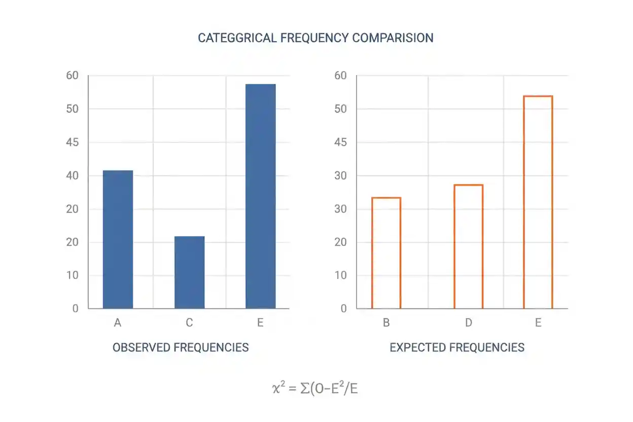
The chi-square test of independence is an inferential statistical procedure used to determine whether two categorical variables are statistically associated in a population. It begins with a contingency table containing observed counts for combinations of categories, such as product preference by region, payment method by customer type, or survey response by age group. Under the null hypothesis, the two variables are treated as independent, meaning the probability distribution of one variable does not systematically change across categories of the other. Expected frequencies are calculated from the row totals, column totals, and overall sample size to represent what the table would look like if independence were true. The observed and expected counts are then compared using a chi-square statistic.
Larger discrepancies produce larger values of χ² and stronger evidence against independence, provided the assumptions of the procedure are reasonably satisfied. The test can establish statistical evidence of association, but it does not establish causation, identify the underlying mechanism, or by itself indicate whether an association is practically important. Correct interpretation therefore requires attention to the sampling design, expected counts, degrees of freedom, p-value, and the actual pattern of differences within the table.
The procedure belongs to Statistics & Probability and forms part of the broader toolkit covered in Inference & Regression. Its specific purpose is to evaluate independence between two categorical variables rather than to test a single categorical distribution or compare quantitative means.
What Is the Chi-Square Test of Independence?
The chi-square test of independence evaluates whether two categorical variables behave independently or show evidence of association. The data are arranged in a contingency table, also called a cross-tabulation, in which rows represent categories of one variable and columns represent categories of the other.
Suppose a researcher records both customer region and preferred payment method. If payment preference is independent of region, the relative distribution of payment methods should be similar across regions apart from random sampling variation. If the observed table differs substantially from what independence predicts, the resulting chi-square statistic can provide evidence that payment preference and region are associated.
The test statistic is:
χ² = Σ[(Oᵢⱼ − Eᵢⱼ)² / Eᵢⱼ]
where Oᵢⱼ is the observed frequency in row i and column j, while Eᵢⱼ is the expected frequency for that cell under the assumption of independence.
The summation includes every cell in the contingency table. Because each difference is squared, positive and negative discrepancies cannot cancel one another. A larger χ² generally means the observed table differs more strongly from the table expected under independence.
Null and Alternative Hypotheses
The null hypothesis for a chi-square test of independence states that the two categorical variables are independent in the population.
In conceptual form:
H₀: Variable A and Variable B are independent.
The alternative hypothesis states that the variables are associated:
H₁: Variable A and Variable B are not independent.
Rejecting H₀ therefore provides evidence of a statistical association between the variables. It does not establish that one variable causes the other. An observed association may reflect causation, reverse causation, confounding, selection effects, measurement processes, or another structural relationship.
Failing to reject H₀ also does not prove independence. It means that the available data do not provide sufficiently strong evidence against independence at the chosen significance level and under the assumptions of the test.
The Contingency Table
A contingency table organizes joint categorical frequencies. Suppose 200 customers are divided between two regions and asked to choose among three products.
| Region | Product A | Product B | Product C | Row Total |
|---|---|---|---|---|
| Region 1 | 40 | 30 | 30 | 100 |
| Region 2 | 20 | 50 | 30 | 100 |
| Column Total | 60 | 80 | 60 | 200 |
The six interior cells are the observed frequencies. The row totals summarize the first variable, while the column totals summarize the second.
The central question is whether the product distribution differs between the two regions more than would reasonably be expected from random sampling variation.
If region and product preference are independent, each region should receive product counts proportional to the overall product frequencies. Those expected frequencies can be calculated entirely from the marginal totals.
Expected Frequency Formula
For each cell in a contingency table:
Eᵢⱼ = (Row Totalᵢ × Column Totalⱼ) / n
where n is the total number of observations.
For Region 1 and Product A:
E₁₁ = (100 × 60) / 200
E₁₁ = 30
Also, For Region 1 and Product B:
E₁₂ = (100 × 80) / 200
E₁₂ = 40
For Region 1 and Product C:
E₁₃ = (100 × 60) / 200
E₁₃ = 30
Because both row totals equal 100, Region 2 has the same expected frequencies: 30, 40, and 30.
The expected table under H₀ is therefore:
| Region | Product A | Product B | Product C |
|---|---|---|---|
| Region 1 | 30 | 40 | 30 |
| Region 2 | 30 | 40 | 30 |
These expected counts represent the frequencies implied by the observed marginal totals if the row variable and column variable are independent.
Why the Expected Frequency Formula Works
Under independence, the joint probability of belonging to row category i and column category j equals the product of the corresponding marginal probabilities. If the proportion of observations in row i is Row Totalᵢ/n and the proportion in column j is Column Totalⱼ/n, independence implies:
P(Row i and Column j) = P(Row i) × P(Column j)
Therefore:
P(Row i and Column j) = (Row Totalᵢ / n) × (Column Totalⱼ / n)
Multiplying this probability by n converts it into an expected count:
Eᵢⱼ = n × (Row Totalᵢ / n) × (Column Totalⱼ / n)
which simplifies to:
Eᵢⱼ = (Row Totalᵢ × Column Totalⱼ) / n
The expected frequencies are thus not arbitrary benchmarks. They follow directly from the assumption that the row and column variables are independent.
Chi-Square Test of Independence Formula
After expected counts are calculated, every observed cell is compared with its expected value using:
χ² = Σ[(Oᵢⱼ − Eᵢⱼ)² / Eᵢⱼ]
A single cell’s contribution is:
χ²ᵢⱼ = (Oᵢⱼ − Eᵢⱼ)² / Eᵢⱼ
The total χ² statistic is obtained by adding the contributions from all cells.
Several features of this formula matter. The observed-minus-expected difference measures deviation from independence. Squaring ensures that departures in opposite directions do not cancel. Dividing by the expected frequency scales each discrepancy relative to the size of the cell expected under H₀.
Because all contributions are nonnegative:
χ² ≥ 0
A value of χ² = 0 occurs only when every observed cell frequency exactly equals its expected frequency under independence.
Worked Example: Product Preference and Region
Return to the customer table:
| Region | Product A | Product B | Product C |
|---|---|---|---|
| Region 1 | 40 | 30 | 30 |
| Region 2 | 20 | 50 | 30 |
The corresponding expected table is:
| Region | Product A | Product B | Product C |
|---|---|---|---|
| Region 1 | 30 | 40 | 30 |
| Region 2 | 30 | 40 | 30 |
Now calculate each contribution.
For Region 1, Product A:
(40 − 30)² / 30 = 100 / 30 ≈ 3.333
For Region 1, Product B:
(30 − 40)² / 40 = 100 / 40 = 2.5
Also, For Region 1, Product C:
(30 − 30)² / 30 = 0
For Region 2, Product A:
(20 − 30)² / 30 = 100 / 30 ≈ 3.333
For Region 2, Product B:
(50 − 40)² / 40 = 100 / 40 = 2.5
Also, For Region 2, Product C:
(30 − 30)² / 30 = 0
Adding all six contributions gives:
χ² ≈ 3.333 + 2.5 + 0 + 3.333 + 2.5 + 0
χ² ≈ 11.667
The statistic shows substantial disagreement between the observed table and the expected frequencies predicted by independence.
Degrees of Freedom
For an r × c contingency table, the degrees of freedom are:
df = (r − 1)(c − 1)
In the example, there are two rows and three columns:
df = (2 − 1)(3 − 1)
df = 1 × 2
df = 2
The degrees of freedom reflect how many cell frequencies can vary independently once the marginal totals constrain the table.
This is different from the simple k − 1 formula often used in a chi-square goodness of fit problem. The two procedures use closely related chi-square statistics, but their table structures, hypotheses, expected-frequency calculations, and degrees of freedom answer different statistical questions.
Finding the P-Value
For the worked example:
χ² ≈ 11.667
df = 2
The upper-tail probability from a chi-square distribution with two degrees of freedom is approximately:
p ≈ 0.00293
The p-value represents the probability, assuming H₀ and the statistical model are correct, of observing a chi-square statistic at least as large as the one calculated.
If the selected significance level is:
α = 0.05
then:
p ≈ 0.00293 < 0.05
The null hypothesis is rejected. The sample provides statistically significant evidence that product preference and region are associated.
This does not mean there is a 0.293% probability that H₀ is true. A frequentist p-value is calculated under the assumption that H₀ is true; it is not a posterior probability assigned to the hypothesis.
Using a Critical Value
The same test can be evaluated with a critical value instead of an exact p-value. For a given α and df, the chi-square distribution provides an upper-tail cutoff.
The decision rule is:
Reject H₀ if χ²observed > χ²critical
For df = 2 and α = 0.05, the critical value is approximately:
χ²critical ≈ 5.991
The observed statistic is:
χ²observed ≈ 11.667
Since:
11.667 > 5.991
the null hypothesis is rejected.
The critical-value approach and the p-value approach are equivalent when they use the same significance level and reference distribution.
What a Significant Result Actually Means
A statistically significant chi-square test of independence means the observed joint distribution is sufficiently inconsistent with independence to reject H₀ at the chosen significance level.
In the product example, Region 1 selected Product A more frequently than predicted by independence and Product B less frequently than predicted. Region 2 displayed the opposite pattern. Product C matched its expected frequency in both regions.
The result therefore suggests that product preference varies with region in the population represented by the sampling process.
It does not show that region directly causes preference. Establishing causation generally requires stronger design and identification assumptions than an association test provides. Randomized experiments, longitudinal structures, control of confounding variables, and substantive causal reasoning may all matter depending on the research question.
Which Cells Drive the Association?
The total χ² statistic combines information across the entire table, but the individual cell contributions can reveal where large observed-versus-expected discrepancies occur.
For the example, the two Product A cells each contribute approximately 3.333, while the two Product B cells each contribute 2.5. The Product C cells contribute zero.
This indicates that the detected association is mainly related to different frequencies of Product A and Product B across the two regions.
A simple Pearson residual for a cell can be written as:
rᵢⱼ = (Oᵢⱼ − Eᵢⱼ) / √Eᵢⱼ
Positive residuals indicate observed counts above expectation, while negative residuals indicate counts below expectation. Their magnitudes can help describe which cells differ most strongly, although formal post-hoc inference can require additional adjustments.
The overall test should remain the primary result. Cell-level interpretation explains the pattern rather than replacing the joint test with a collection of uncorrected individual comparisons.
Assumptions of the Chi-Square Test of Independence
The procedure works best when the data meet several important conditions. First, both variables should be categorical. The categories may be nominal, such as product type or color, or ordered, such as satisfaction levels, although the ordinary Pearson test does not use the ordering information.
Second, observations should be appropriately independent. Each sampling unit should contribute to one cell of the contingency table. Recording the same participant multiple times as though each response were an independent person can distort the sampling variation and invalidate the ordinary calculation.
Third, categories should be mutually exclusive within each variable. An observation must have a clearly defined row category and column category.
Fourth, expected counts must be large enough for the chi-square reference distribution to provide a reasonable approximation. Small or sparse expected frequencies can cause the asymptotic distribution to approximate the true finite-sample behavior poorly.
Finally, the sampling process itself matters. A mathematically correct χ² calculation cannot repair severe selection bias, dependence, measurement error, or a sample that does not meaningfully represent the target population.
Expected Count Requirements
A common introductory guideline recommends expected cell frequencies of approximately 5 or greater. This is useful as a rough diagnostic, but it should not be treated as an absolute universal theorem.
A 2 × 2 table with small expected frequencies may require an exact method rather than the standard asymptotic chi-square approximation. In larger tables, the distribution of small expected cells across the table also matters.
The important principle is that the chi-square test relies on an approximation to a theoretical sampling distribution. Sparse data can weaken that approximation.
Combining categories merely to satisfy a numerical rule is not automatically appropriate. Categories should only be combined when the merged categories remain substantively meaningful.
Independence of Observations vs Independence of Variables
The word independence appears in two different roles and should not be confused.
Independence of observations is an assumption about the sampling units. It means the observations provide appropriately separate information for the ordinary test.
Independence of variables is the null hypothesis being tested.
A dataset can contain independent observations while the two variables are strongly associated. For example, 1,000 independently sampled customers may show a clear relationship between region and product preference.
Conversely, the variables might truly be independent while the observations themselves are clustered or repeated. In that case, the standard Pearson test may still be inappropriate because its sampling assumptions are violated.
Sampling Distribution of the Statistic
The logic of the procedure is based on the sampling distribution of the χ² statistic under H₀. Imagine repeatedly drawing samples from a population in which the two variables are genuinely independent. Each sample produces slightly different observed counts because of random sampling variation, and therefore each sample produces a different χ² statistic.
When the required conditions are sufficiently satisfied, the distribution of those statistics is approximately a chi-square distribution with:
df = (r − 1)(c − 1)
The observed χ² value is evaluated relative to that reference distribution. Very large values fall into its upper tail and indicate discrepancies greater than would usually be expected when independence is true.
Large-sample distribution theory, including ideas related to the central limit theorem, helps explain why many inferential statistics have useful asymptotic reference distributions. The chi-square test nevertheless has its own derivation and should not be reduced to the sample-mean CLT formula.
Chi-Square Test of Independence vs Goodness of Fit
The chi-square test of independence and chi-square goodness of fit both use Pearson-style observed-versus-expected calculations, but they own different statistical questions.
A goodness of fit test studies one categorical variable. It asks whether its observed category frequencies match a specified probability distribution.
A test of independence studies two categorical variables. It asks whether their joint distribution is consistent with statistical independence.
For goodness of fit, expected probabilities are generally specified by H₀ or estimated according to a particular model. For independence, expected cell frequencies are obtained from the row and column marginal totals:
Eᵢⱼ = (Row Totalᵢ × Column Totalⱼ) / n
Use the chi-square goodness of fit procedure when the question concerns whether one variable follows a stated distribution. Use the independence test when the question concerns association between two categorical variables.
Chi-Square Independence vs Correlation
Both association and correlation describe relationships, but they are not interchangeable statistical concepts. The ordinary chi-square test of independence is designed for categorical variables and asks whether the joint frequency structure is consistent with independence.
Correlation typically quantifies a particular form of relationship between numerical variables, especially linear association when Pearson correlation is used. Converting categories into arbitrary numbers and treating those codes as quantitative values can create misleading results.
A significant chi-square test therefore should usually be described as evidence of association rather than as evidence of “correlation” unless a separate correlation measure is genuinely appropriate for the variables involved.
Neither association nor correlation by itself establishes causation.
Chi-Square Independence vs Regression Measures
The coefficient of determination belongs to regression analysis and commonly describes the proportion of variation in an outcome associated with a fitted model under its relevant definition. It does not serve the same purpose as the chi-square independence statistic.
A χ² value is not a percentage of variance explained. Likewise, a large χ² value should not be interpreted as a larger R².
The chi-square test asks whether categorical variables are independent. Regression methods can address different questions, potentially including prediction, adjustment for multiple variables, and estimation of conditional relationships. A simple contingency-table test should not be stretched into those broader roles.
Statistical Significance vs Strength of Association
The chi-square statistic and its p-value determine whether the data provide evidence against independence, but they do not by themselves give a standardized description of how strong the association is.
This distinction becomes especially important with large samples. A huge dataset can detect a small departure from independence that is statistically compelling but practically unimportant.
An effect size can provide complementary information about magnitude. For contingency tables, measures such as Cramér’s V are often used to summarize association strength.
For a table with r rows and c columns, Cramér’s V can be written as:
V = √[χ² / (n × min(r − 1, c − 1))]
Its value ranges from 0 to 1 in the usual setting, with 0 representing no observed association according to this measure and larger values representing stronger association.
The substantive meaning of a particular value depends on the field, variables, study design, and consequences involved. Universal labels such as “small” or “large” should therefore be used cautiously.
Why Cohen D Is Different
Cohen D is a standardized effect-size measure typically used to express a difference between quantitative group means. It is not the ordinary association measure for a contingency table.
For two categorical variables, Cramér’s V, the phi coefficient in an appropriate 2 × 2 setting, odds ratios for certain designs, or other categorical association measures may be more meaningful depending on the problem.
This distinction illustrates a broader rule: effect-size measures are tied to particular data structures and questions. Statistical significance should not be supplemented with an unrelated effect-size formula merely because both are numerical summaries.
Sample Size and Statistical Significance
The chi-square statistic is sensitive to sample size because observed-minus-expected differences can become increasingly detectable as n grows.
Suppose two variables have only a slight association. In a sample of 100 observations, the resulting discrepancy may be difficult to distinguish from ordinary sampling variability. In a sample of 100,000 observations, essentially the same proportional difference can produce a very small p-value.
This does not mean the relationship became practically stronger solely because the sample grew. It means the estimate became precise enough to detect a smaller departure from independence.
That is why reporting only the p-value can be misleading. The observed proportions, sample size, direction of differences, and relevant association magnitude should also be considered.
Type I Error
A Type I error occurs when the researcher rejects the null hypothesis of independence even though the variables are actually independent in the population.
If the significance level is α = 0.05 and the test assumptions hold, the testing procedure is constructed so that the long-run probability of rejecting a true H₀ is 5%.
This does not mean every significant result has a 5% probability of being wrong. The significance level describes the repeated-sampling behavior of the procedure under H₀ rather than the posterior probability of a particular conclusion.
Statistical Power
Statistical power is the probability that a test rejects H₀ when a specified alternative relationship actually exists. Power generally increases when the sample size grows, the association becomes stronger, or the data structure provides clearer information.
A nonsignificant result in a low-powered study can therefore occur even when the variables are genuinely associated. This is another reason that failing to reject H₀ should not be described as proof that the variables are independent.
Power depends on the size and pattern of the departure from independence, the sample size, table dimensions, significance level, and other features of the design.
Worked Example: A 2 × 2 Table
Suppose 300 people are classified according to whether they received a particular communication and whether they completed an action.
| Group | Completed | Did Not Complete | Total |
|---|---|---|---|
| Received | 90 | 60 | 150 |
| Not Received | 60 | 90 | 150 |
| Total | 150 | 150 | 300 |
Under independence, the expected count for the Received–Completed cell is:
E = (150 × 150) / 300 = 75
Because the row and column totals are balanced, all four expected counts equal 75.
The chi-square statistic is:
χ² = (90 − 75)²/75 + (60 − 75)²/75 + (60 − 75)²/75 + (90 − 75)²/75
Each contribution is:
225 / 75 = 3
Therefore:
χ² = 3 + 3 + 3 + 3 = 12
The degrees of freedom are:
df = (2 − 1)(2 − 1) = 1
This χ² value would produce strong evidence against independence under the ordinary Pearson approximation. The table suggests that completion status differs across the two groups.
However, this result alone does not establish that receiving the communication caused the difference. That causal interpretation would depend on how people entered the groups, whether assignment was randomized, whether confounding variables were controlled, and whether the measurements were valid.
When the Chi-Square Approximation Can Be Poor
The standard approximation can be unreliable when expected counts are very small, the sample is sparse, observations are dependent, or the table contains structural features inconsistent with the ordinary multinomial framework.
Rare categories can be especially problematic. Suppose one column contains only two observations in the entire dataset. The expected frequencies for that column may be extremely small across several rows, leaving little basis for an asymptotic chi-square approximation.
The approximation also does not fix sampling problems. Thousands of observations collected from a biased or non-independent process can generate an extremely precise answer to the wrong population question.
A larger n helps with some approximation issues, but sample size should never be treated as a universal substitute for appropriate study design.
Missing Data and Category Definitions
The validity of a contingency table depends on how observations are categorized. Ambiguous, overlapping, or inconsistently applied categories can introduce measurement error before the test is even calculated.
Missing observations can also matter when the probability of missingness is related to either categorical variable. Simply discarding incomplete cases may change the composition of the analyzed sample and potentially alter the observed association.
The chi-square formula assumes that the table supplied to it meaningfully represents the data-generating process. Statistical calculations cannot compensate for poorly defined variables.
Common Misconceptions
One common misconception is that a significant chi-square test proves that one variable causes the other. It does not. The test identifies statistical association, not causal direction or mechanism.
Another mistake is interpreting the p-value as the probability that the variables are independent. A p-value is calculated under H₀ and describes the extremeness of the observed statistic relative to its null reference distribution.
A third misconception is that a larger χ² automatically means a stronger association. The raw statistic depends on sample size, table structure, and the magnitude of the discrepancies. Association strength should be evaluated with an appropriate effect-size measure and the actual observed proportions.
Researchers also sometimes use the test on percentages without access to the underlying counts. The Pearson statistic is fundamentally based on frequencies, and sample size affects both expected counts and statistical significance.
Finally, a nonsignificant result does not prove independence. It means the available evidence was insufficient to reject the independence model under the selected procedure.
How to Perform a Chi-Square Test of Independence
Begin with two categorical variables measured on a sample of observational units. Arrange the joint frequencies into an r × c contingency table and calculate the row totals, column totals, and overall total n.
State:
H₀: the variables are independent.
H₁: the variables are associated.
Next calculate each expected frequency:
Eᵢⱼ = (Row Totalᵢ × Column Totalⱼ) / n
Check whether the expected frequencies and sampling design make the ordinary chi-square approximation reasonable. Then calculate:
χ² = Σ[(Oᵢⱼ − Eᵢⱼ)² / Eᵢⱼ]
Determine:
df = (r − 1)(c − 1)
Use the chi-square reference distribution to obtain a p-value or compare the statistic with a critical value. Finally, interpret the conclusion in the context of the variables while separating evidence of association from claims about causation or practical importance.
How to Report the Result
A concise report should identify the variables, the chi-square statistic, degrees of freedom, sample size, p-value, and contextual conclusion.
For the product-preference example, a suitable interpretation is:
Product preference was associated with region, χ²(2) ≈ 11.67, p ≈ 0.0029.
The substantive explanation can then state that Product A was observed more frequently than expected in Region 1 and less frequently than expected in Region 2, while Product B showed the reverse pattern.
Avoid statements such as “region caused product preference” unless the research design independently supports a causal conclusion.
Frequently Asked Questions
What does the chi-square test of independence test?
It tests whether two categorical variables are statistically independent in the population represented by the sampling process. A significant result provides evidence that the variables are associated.
What is the chi-square test of independence formula?
The Pearson statistic is:
χ² = Σ[(Oᵢⱼ − Eᵢⱼ)² / Eᵢⱼ]
where Oᵢⱼ is an observed cell count and Eᵢⱼ is the expected count under independence.
How do you calculate an expected frequency?
For a cell in row i and column j:
Eᵢⱼ = (Row Totalᵢ × Column Totalⱼ) / n
This formula follows from the null hypothesis that the two categorical variables are independent.
What is the null hypothesis?
The null hypothesis states that the row variable and column variable are independent in the population.
What is the alternative hypothesis?
The alternative states that the variables are not independent, meaning there is some association between them.
How do you calculate degrees of freedom?
For an r × c table:
df = (r − 1)(c − 1)
A 2 × 3 table therefore has 2 degrees of freedom.
What does a large chi-square statistic mean?
A large χ² indicates that the observed cell frequencies differ substantially from the counts expected under independence. Whether the difference is statistically significant depends on the degrees of freedom and reference distribution.
Can chi-square be negative?
No. The statistic is a sum of squared deviations divided by positive expected frequencies, so:
χ² ≥ 0
Does a significant chi-square test prove causation?
No. It provides evidence of association between categorical variables. Causal conclusions require additional assumptions and an appropriate research design.
What is the difference between chi-square independence and goodness of fit?
A goodness of fit test examines whether one categorical variable follows a specified distribution. A test of independence examines whether two categorical variables are associated.
Can the test be used with quantitative variables?
Not directly in its ordinary form. It is designed for categorical frequency data. Converting quantitative measurements into categories may discard useful information and should only be done when substantively justified.
What happens if expected counts are too small?
The ordinary chi-square approximation may become unreliable. An exact or alternative procedure may be preferable depending on the size and structure of the contingency table.
Is a p-value the probability that the variables are independent?
No. The p-value is calculated assuming independence and measures how extreme the observed test statistic would be under that assumption.
Does a larger sample always mean a stronger association?
No. Larger samples make smaller associations easier to detect statistically. Strength of association and statistical significance are separate concepts.
What should be examined after a significant result?
Examine the observed and expected frequencies, cell contributions or residual patterns, and an appropriate measure of association strength. These help explain where and how the variables differ from independence.
Key Takeaway
The chi-square test of independence determines whether two categorical variables show evidence of statistical association. It compares observed cell frequencies with frequencies predicted under the null hypothesis of independence:
Eᵢⱼ = (Row Totalᵢ × Column Totalⱼ) / n
The resulting discrepancies are summarized by:
χ² = Σ[(Oᵢⱼ − Eᵢⱼ)² / Eᵢⱼ]
with degrees of freedom:
df = (r − 1)(c − 1)
A sufficiently large χ² and correspondingly small p-value provide evidence against independence. The conclusion is about statistical association—not causation—and should be interpreted alongside the sampling design, expected counts, observed proportions, and an appropriate measure of association magnitude. Used within those boundaries, the chi-square test of independence provides a clear and practical framework for analyzing relationships between categorical variables.



