
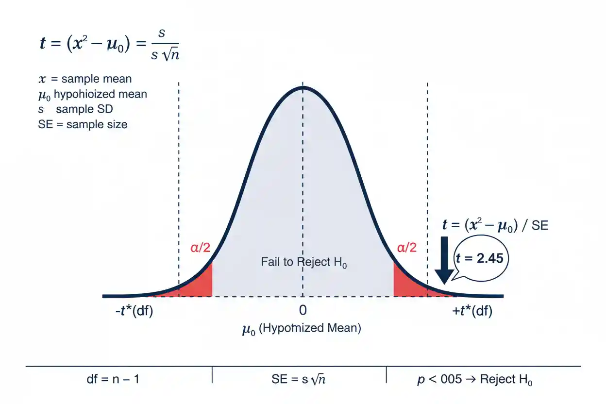

The one-sample t-test is an inferential statistical procedure used to evaluate whether the mean of a population differs from a specified reference value when the population standard deviation is unknown. It compares the observed sample mean with the hypothesized population mean and scales their difference by the estimated standard error of the sample mean. The resulting t statistic measures how many estimated standard errors separate the observed mean from the value specified by the null hypothesis. Because the population standard deviation must be estimated from the sample, the test uses Student’s t distribution rather than automatically using the standard normal distribution.
The shape of that reference distribution depends on the sample’s degrees of freedom, which for the standard one-sample procedure equal n − 1. The test can be two-sided when departures in either direction matter or one-sided when the research question specifies a direction in advance. A statistically significant result indicates evidence against the specified population mean, but it does not determine whether the observed difference is practically important. Correct use also depends on the sampling design, independence of observations, behavior of the outcome distribution, and the absence of extreme influential observations that make mean-based inference unreliable.
The one-sample t-test is part of Statistics & Probability and the broader Inference & Regression framework. It provides a focused method for testing a single population mean rather than the multi-predictor relationships addressed by Multiple Regression or binary-outcome modeling handled by Logistic Regression.
What Is a One-Sample T-Test?
A one-sample t-test compares the mean calculated from one sample with a hypothesized population mean μ₀. The central question is whether the observed difference between x̄ and μ₀ is large relative to the amount of sampling variability expected when the null hypothesis is true.
The basic hypotheses for a two-sided test are:
H₀: μ = μ₀
H₁: μ ≠ μ₀
The Null Hypothesis specifies the population mean used as the reference benchmark. The test does not begin by asking whether μ₀ looks plausible from the raw difference alone. Instead, it evaluates the difference relative to the estimated standard error.
The one-sample t statistic is:
t = (x̄ − μ₀) / (s / √n)
where:
- x̄ = sample mean
- μ₀ = hypothesized population mean
- s = sample standard deviation
- n = sample size
The denominator:
s / √n
is the estimated standard error of the sample mean.
One-Sample T-Test Formula
The core formula is:
t = (x̄ − μ₀) / SE(x̄)
with:
SE(x̄) = s / √n
Therefore:
t = (x̄ − μ₀) / (s / √n)
The numerator measures the raw difference between the sample mean and the null value:
Difference = x̄ − μ₀
The denominator expresses the estimated sampling variability of x̄.
This means the test does not ask only whether the observed mean differs from μ₀. It asks whether the difference is large enough relative to the uncertainty in the sample mean to be difficult to explain through sampling variation under H₀.
For example, a five-unit difference can generate strong statistical evidence when the standard error is 1 but weak evidence when the standard error is 10.
Degrees of Freedom
For the ordinary one-sample t-test:
df = n − 1
If:
n = 20
then:
df = 19
If:
n = 100
then:
df = 99
The loss of one degree of freedom occurs because the sample mean is estimated from the same observations used to calculate the sample variance. Once deviations from the sample mean are determined for n − 1 observations, the final deviation is constrained by the requirement that deviations from x̄ sum to zero.
The degrees of freedom determine the exact Student’s t reference distribution used for the test.
Why Use the t Distribution?
If the population standard deviation σ were known and the relevant conditions for a z procedure were satisfied, the standardized sample mean could use:
z = (x̄ − μ₀) / (σ / √n)
In most practical situations, however, σ is unknown. The sample standard deviation s must be substituted for σ:
SE(x̄) = s / √n
Estimating σ introduces additional uncertainty. Student’s t distribution accounts for that uncertainty by having heavier tails than the standard normal distribution, especially when df is small.
As df increases, the t distribution becomes increasingly similar to the standard normal distribution:
t distribution → standard normal distribution as df increases
This is why t critical values are relatively large for small samples but approach corresponding z critical values for large samples.
The related known-σ procedure is covered separately in the One-Sample Z-Test.
Worked Example: Two-Sided One-Sample T-Test
Suppose a manufacturing process is designed to produce components with an average measurement of 50 units. A random sample gives:
n = 25
x̄ = 53
s = 5
The research question asks whether the population mean differs from 50 in either direction.
The hypotheses are:
H₀: μ = 50
H₁: μ ≠ 50
First calculate the estimated standard error:
SE(x̄) = s / √n
SE(x̄) = 5 / √25
SE(x̄) = 5 / 5
SE(x̄) = 1
Now calculate the t statistic:
t = (53 − 50) / 1
t = 3
The degrees of freedom are:
df = 25 − 1
df = 24
For a two-sided test with:
α = 0.05
and:
df = 24
the critical values are approximately:
±2.064
Because:
|3| > 2.064
the observed statistic falls inside the rejection region.
The null hypothesis is rejected at the 5% significance level. The sample provides statistical evidence that the population mean differs from 50.
Interpreting the Worked Example
The sample mean exceeds the hypothesized mean by:
53 − 50 = 3
The estimated standard error is:
1
Therefore, the observed sample mean lies:
3 standard errors
above the null value.
That standardized distance is what creates the t statistic of 3.
The conclusion should not be stated as “there is a 95% probability that the true mean differs from 50.” A frequentist t-test does not assign that probability to the parameter or hypothesis.
It is also not enough to say that the result is significant. Whether a three-unit difference matters in practice depends on the measurement scale, tolerances, costs, and consequences associated with the process.
P-Value Interpretation
The p-value is the probability, under H₀ and the statistical model, of obtaining a t statistic at least as extreme as the observed statistic according to the chosen test direction.
For a two-sided test:
p-value = P(|T| ≥ |tobserved| | H₀)
For the worked example:
tobserved = 3
df = 24
The two-sided p-value is approximately:
p ≈ 0.006
At:
α = 0.05
we have:
p < α
so H₀ is rejected.
The p-value is not the probability that H₀ is true. It is calculated conditional on the null hypothesis.
Critical-Value Decision Rule
A one-sample t-test can also be conducted by comparing the observed statistic directly with a critical value.
For a symmetric two-sided test:
Reject H₀ if |tobserved| > tcritical
Suppose:
tobserved = 3.00
and:
tcritical = 2.064
Then:
3.00 > 2.064
so H₀ is rejected.
If instead:
tobserved = 1.50
then:
1.50 < 2.064
and H₀ would not be rejected.
The critical-value and p-value methods produce the same decision when the same test, degrees of freedom, and α are used.
Two-Sided One-Sample T-Test
A two-sided test is appropriate when differences above and below μ₀ are both relevant.
The hypotheses are:
H₀: μ = μ₀
H₁: μ ≠ μ₀
If:
α = 0.05
the rejection probability is divided between both tails of the t distribution:
α/2 = 0.025
in each tail.
The rejection rule becomes:
t < −tcritical or t > tcritical
Equivalently:
|t| > tcritical
A two-sided test should generally be used when the research question concerns any departure from the reference value rather than one specifically predicted direction.
Right-Tailed One-Sample T-Test
A right-tailed test is used when the question asks whether the population mean is greater than the reference value.
For example:
H₀: μ = 100
H₁: μ > 100
The rejection region lies entirely in the upper tail.
At:
α = 0.05
the critical value is the point leaving 5% of the relevant t distribution above it.
The decision rule is:
Reject H₀ if tobserved > tcritical
A positive statistic supports the direction of H₁, but it must still be sufficiently large to cross the inferential threshold.
The right-tailed alternative should follow from the research question before inspecting whether the observed sample mean happens to be above μ₀.
Left-Tailed One-Sample T-Test
A left-tailed test is appropriate when the alternative states that the population mean is below the reference value.
The hypotheses can be written:
H₀: μ = μ₀
H₁: μ < μ₀
The rejection region lies in the lower tail.
The decision rule is:
Reject H₀ if tobserved < tcritical
where tcritical is negative.
For example, if:
tcritical = −1.729
and:
tobserved = −2.4
then:
−2.4 < −1.729
and H₀ is rejected.
Again, the test direction should be established by the substantive hypothesis rather than chosen after seeing the sign of x̄ − μ₀.
Worked Example: Right-Tailed Test
Suppose a training program is expected to raise a performance measure above a historical benchmark of 70.
A sample produces:
n = 16
x̄ = 74
s = 8
The hypotheses are:
H₀: μ = 70
H₁: μ > 70
Calculate the standard error:
SE(x̄) = 8 / √16
SE(x̄) = 8 / 4
SE(x̄) = 2
Then:
t = (74 − 70) / 2
t = 2
The degrees of freedom are:
df = 16 − 1
df = 15
For a right-tailed test with α = 0.05 and df = 15, the critical value is approximately:
tcritical ≈ 1.753
Because:
2 > 1.753
the test rejects H₀ at the 5% significance level.
The sample provides evidence that the population mean exceeds 70 under the assumptions of the procedure.
Confidence Interval Connection
A one-sample t-test is closely connected with a t-based confidence interval for the population mean.
A common interval is:
x̄ ± t* × s / √n
where t* is the critical value associated with the chosen confidence level and df = n − 1.
For the earlier example:
x̄ = 53
s = 5
n = 25
df = 24
For a 95% confidence interval:
t* ≈ 2.064
The standard error is:
1
so the margin of error is:
2.064 × 1 = 2.064
The interval is:
53 ± 2.064
giving:
Lower ≈ 50.936
Upper ≈ 55.064
The null value 50 lies outside this interval, which is consistent with rejecting H₀: μ = 50 in the corresponding two-sided α = 0.05 test.
What a Confidence Interval Adds
The hypothesis test answers whether the sample provides sufficient evidence against one specified null value. The confidence interval provides a range of population means compatible with the observations under the interval procedure and model assumptions.
In the previous example, rejecting:
H₀: μ = 50
tells us that 50 is outside the corresponding 95% interval.
The interval:
approximately 50.94 to 55.06
also indicates the magnitude and uncertainty of the estimated population mean.
This is often more informative than reporting only “statistically significant.”
A conventional frequentist 95% confidence interval does not mean there is a 95% posterior probability that μ lies between those particular observed endpoints.
Assumptions of the One-Sample T-Test
The standard one-sample t-test rests on several conditions that concern the measurement scale, sampling structure, and distribution of observations.
The outcome should be quantitative so that a population mean and standard deviation are meaningful. Observations should provide appropriately independent information. The sample should arise from a design that supports inference to the target population. Extreme outliers deserve particular attention because both the sample mean and sample standard deviation are sensitive to them.
For exact small-sample t inference, the classical model assumes the observations come from a normally distributed population. With larger samples, the sampling distribution of the mean can often be approximately normal even when the population itself is not perfectly normal, but the approximation quality depends on the underlying distribution.
There is no universal sample size at which distributional concerns disappear.
Independence of Observations
Independence is fundamental to the ordinary standard-error formula:
SE(x̄) = s / √n
If the observations are strongly dependent, this formula may understate or otherwise misrepresent the actual sampling variability.
For example, repeatedly measuring the same person and pretending that every measurement comes from a different independent participant can artificially inflate the apparent sample size.
Likewise, students within one classroom, employees within one team, or measurements collected over time may contain dependence.
A larger number of correlated observations does not automatically solve the problem. The analytical method must reflect the dependence structure.
Random Sampling and Generalization
A one-sample t calculation can be performed on almost any numerical dataset, but the validity of population inference depends on how the observations were obtained.
A genuinely random or otherwise defensible sampling mechanism supports broader generalization. A convenience sample may accurately describe itself while providing limited evidence about a larger target population.
For example, a sample of customers who voluntarily respond to a survey may differ systematically from all customers.
The t-test cannot mathematically correct a biased sampling process simply by producing a small p-value.
Sampling design and statistical calculation therefore answer different parts of the inferential problem.
Normality and the One-Sample T-Test
The exact classical one-sample t distribution arises when the observations are independent draws from a normal population with unknown variance.
That does not mean the raw sample must look perfectly bell-shaped for every practical use.
The t-test is often reasonably robust to mild deviations from normality, especially when the sample is not tiny and the outcome lacks severe skewness or extreme outliers. As n increases, the sampling distribution of x̄ may become more nearly normal under finite-variance conditions.
However, strong skewness, extremely heavy tails, or rare extreme observations can make convergence slow. A large sample should therefore not be treated as a universal license to ignore data behavior.
There Is No Universal n = 30 Rule
A frequent misconception is that the t-test becomes automatically valid when:
n ≥ 30
No theorem establishes 30 as a universal cutoff.
For a symmetric, well-behaved distribution, a sample smaller than 30 may support useful t inference. For a severely skewed or heavy-tailed population, even a substantially larger sample can produce an unstable sample mean or poor approximation.
Sample-size adequacy depends on:
- skewness
- tail behavior
- outliers
- dependence
- required accuracy
- sampling design
The number 30 can occasionally serve as a rough classroom heuristic, but it should not replace evaluation of the actual statistical conditions.
Outliers Matter
The sample mean is sensitive to extreme values, and so is the sample standard deviation used in the t statistic.
Suppose most observations lie between 45 and 55 but one observation equals 500. That single value can dramatically increase both x̄ and s.
Its effect on the t statistic is therefore not always obvious: it may increase the numerator, the denominator, or both.
A one-sample t-test should not proceed mechanically without examining whether unusual observations are genuine measurements, data-entry errors, or evidence that the population is poorly summarized by a mean.
Valid observations should not be removed solely because they prevent a statistically significant result.
One-Sample T-Test vs One-Sample Z-Test
The one-sample t-test and One-Sample Z-Test evaluate similar mean hypotheses but use different standardization assumptions.
The classical t statistic is:
t = (x̄ − μ₀) / (s / √n)
The classical z statistic when population σ is known is:
z = (x̄ − μ₀) / (σ / √n)
The distinction is therefore:
t-test uses sample standard deviation s
z-test uses known population standard deviation σ
Because s is estimated, the t procedure accounts for the additional uncertainty through Student’s t distribution.
As df becomes large, the t and standard normal distributions become very similar.
The choice should follow the statistical conditions rather than a rule stating that z tests are for large samples and t-tests are only for small samples.
The T-Test Is Not Only for Small Samples
Another common misconception is:
small sample → t-test
large sample → z-test
This is incomplete.
If σ is unknown—which is common—the standard one-sample t procedure remains appropriate even with a large sample. With large df, the t distribution becomes so close to the standard normal distribution that the resulting calculations may be numerically similar.
The defining issue is primarily how the standard error is constructed and which reference distribution follows from that uncertainty, not whether n crosses an arbitrary threshold.
Sample Mean vs Population Mean
The sample mean:
x̄
is a statistic calculated from observed data.
The population mean:
μ
is a parameter describing the population of interest.
The one-sample t-test uses x̄ to evaluate a claim about μ.
This distinction is essential. A sample mean of exactly 50 does not prove that:
μ = 50
because another sample will generally produce a different x̄.
Likewise, a sample mean of 52 does not automatically prove:
μ ≠ 50
because random sampling variation can generate differences between x̄ and μ even when the null hypothesis is true.
The test quantifies how unusual the observed discrepancy is relative to estimated sampling variability.
Standard Deviation vs Standard Error
The sample standard deviation s describes variability among individual observations.
The standard error:
SE(x̄) = s / √n
estimates variability among sample means across repeated samples.
These quantities have different interpretations.
Suppose:
s = 20
and:
n = 100
Then:
SE(x̄) = 20 / 10
SE(x̄) = 2
Individual observations vary on a scale of about 20 units, while repeated sample means of size 100 vary on a much smaller scale.
The t-test uses the standard error because its purpose is to evaluate uncertainty in x̄ as an estimate of μ.
Effect of Sample Size
For a fixed sample standard deviation:
SE(x̄) = s / √n
so increasing n reduces the standard error.
If n rises by a factor of four:
√(4n) = 2√n
and the standard error is approximately halved.
This means that a given raw difference:
x̄ − μ₀
produces a larger absolute t statistic when the standard error becomes smaller.
Consequently, large samples can detect smaller departures from H₀.
That increase in statistical sensitivity does not make those departures more practically important. It simply means the mean is estimated with greater precision.
Statistical Significance vs Practical Importance
Suppose a sample of 100,000 observations produces:
x̄ − μ₀ = 0.1
If the standard error is extremely small, the resulting t statistic can be very large and the p-value extremely small.
The test may strongly reject H₀ even though the actual difference is only one-tenth of a unit.
Conversely, a small sample may show:
x̄ − μ₀ = 10
but have such a large standard error that H₀ is not rejected.
The first result may be statistically compelling but practically trivial. The second may suggest a large possible effect but contain substantial uncertainty.
Inferential evidence and practical magnitude should therefore be reported separately.
Effect Size for a One-Sample Mean
A standardized measure can complement the t-test by expressing the sample mean difference relative to the sample standard deviation.
A common one-sample standardized difference is:
d = (x̄ − μ₀) / s
Suppose:
x̄ = 53
μ₀ = 50
s = 5
Then:
d = 3 / 5
d = 0.60
The observed mean is 0.60 sample standard deviations above the reference value.
This standardized magnitude is not the same as the t statistic.
Indeed:
t = d√n
for the corresponding one-sample definitions.
With:
d = 0.60
and:
n = 25
we have:
t = 0.60 × 5
t = 3
The effect-size measure and t statistic are mathematically related but answer different interpretive questions.
Type I Error
A Type I error occurs when H₀ is rejected even though it is true.
At significance level:
α = 0.05
a correctly calibrated procedure has a 5% probability of rejecting the null when the null model is true, under repeated sampling and the required assumptions.
This does not mean that after rejecting H₀ there is a 5% probability the conclusion is wrong.
The 5% rate describes the long-run behavior of the testing procedure under H₀.
Choosing a smaller α reduces this particular false-positive probability but also makes rejection more difficult.
Type II Error and Power
A Type II error occurs when the test fails to reject H₀ even though a relevant alternative is true.
The probability of correctly rejecting H₀ under a specified alternative is statistical power.
Power generally increases when:
- the true difference from μ₀ is larger
- n increases
- variability decreases
- α increases
- the design provides more independent information
This explains why a nonsignificant one-sample t-test does not establish that μ exactly equals μ₀.
The sample may simply lack enough information to distinguish the true mean from the null value.
A Nonsignificant Result Does Not Prove Equality
Suppose the estimated mean is:
x̄ = 101
and the reference value is:
μ₀ = 100
but the 95% confidence interval is:
90 to 112
Because the interval includes 100, the corresponding two-sided test will not reject H₀ at α = 0.05.
However, the same interval also includes population means meaningfully below and above 100.
The data therefore do not demonstrate exact equality. They are simply too imprecise to exclude the null value.
If the goal is to demonstrate that the population mean is sufficiently close to a reference value, an equivalence procedure designed around a prespecified practical margin is more appropriate.
One-Sample T-Test vs Comparing Several Means
The one-sample t-test owns a narrow inferential question: whether one population mean differs from one specified reference value.
When the objective is to compare several independent group means simultaneously, repeatedly applying separate one-sample or pairwise t-tests can create a different inferential problem and potentially inflate error rates.
Methods such as One-Way ANOVA are designed for testing whether several population group means satisfy a common equality structure.
The one-sample t-test should therefore remain focused on a single population mean and a fixed benchmark rather than being expanded into a general multi-group comparison procedure.
T-Test and Regression Connection
Although the one-sample t-test is not a multiple regression procedure, it can be represented within a simple intercept-only linear-model framework.
Consider:
Yᵢ = β₀ + εᵢ
Testing whether the population mean equals μ₀ is equivalent to testing:
H₀: β₀ = μ₀
in this intercept-only model.
This connection helps explain why t statistics appear broadly throughout linear modeling.
However, the one-sample t-test is best interpreted directly as a procedure for a single population mean. Broader coefficient structures, multiple predictors, interactions, and conditional relationships belong to regression analysis rather than this page’s core intent.
When Not to Use a One-Sample T-Test
The procedure is not appropriate when the primary outcome is categorical rather than quantitative.
It is also not the ordinary choice when the observations form paired before-and-after measurements and the target parameter concerns within-pair changes; that design has a different natural data structure.
If multiple independent groups are being compared, a multi-group method may be more appropriate.
If observations are strongly dependent, standard one-sample formulas can give misleading standard errors.
If extreme skewness, heavy tails, or severe outliers make the population mean unstable or unrepresentative, another estimand or inference method may better match the research question.
The correct statistical method follows from the parameter, design, and data-generating process.
Common Mistakes
A common mistake is using the one-sample t-test simply because n is below 30. Sample size alone does not define the test.
Another error is switching automatically to a z-test once n exceeds 30. If σ remains unknown, the t framework is still appropriate.
Researchers also sometimes interpret a nonsignificant result as proof that the population mean equals μ₀. Failure to reject does not establish exact equality.
A further mistake is treating p < 0.05 as evidence that the difference must be practically important. Statistical significance describes evidence relative to sampling uncertainty, not the consequence of the effect.
The t statistic itself is also sometimes confused with the raw mean difference. A t value of 3 does not mean the sample mean differs by three original measurement units; it means the difference equals three estimated standard errors.
Finally, observations should not be treated as independent simply because they appear as separate rows in a dataset.
How to Perform a One-Sample T-Test
Begin by defining the population parameter and reference value:
H₀: μ = μ₀
Then specify whether the alternative is two-sided, right-sided, or left-sided according to the research question.
Calculate the sample mean:
x̄ = Σxᵢ / n
Calculate the sample standard deviation s and estimated standard error:
SE(x̄) = s / √n
Then calculate:
t = (x̄ − μ₀) / (s / √n)
Determine the degrees of freedom:
df = n − 1
Use the appropriate Student’s t distribution to obtain the p-value or critical value.
Finally, interpret the result in terms of the population mean while also reporting the observed difference and uncertainty where possible.
How to Report the Result
A clear report should include the sample mean, reference mean, estimated difference, t statistic, degrees of freedom, and p-value or confidence interval.
For the worked example:
x̄ = 53
μ₀ = 50
t(24) = 3.00
p ≈ 0.006
A concise interpretation is that the sample provides statistically significant evidence that the population mean differs from 50.
Including the estimated difference:
3 units
and the confidence interval for μ provides readers with information about magnitude and uncertainty rather than reporting only the significance decision.
Frequently Asked Questions
What is a one-sample t-test?
A one-sample t-test evaluates whether a population mean differs from a specified reference value when the population standard deviation is unknown and estimated from the sample.
What is the formula for a one-sample t-test?
The test statistic is:
t = (x̄ − μ₀) / (s / √n)
What does x̄ represent?
x̄ is the sample mean calculated from the observed data.
What does μ₀ represent?
μ₀ is the population mean specified by the null hypothesis.
What is the standard error in a one-sample t-test?
The estimated standard error is:
SE(x̄) = s / √n
What are the degrees of freedom?
For the standard one-sample t-test:
df = n − 1
Why does the test use Student’s t distribution?
Because the unknown population standard deviation is estimated with the sample standard deviation, creating additional uncertainty that the t distribution accounts for.
What is the null hypothesis?
A common null is:
H₀: μ = μ₀
It states that the population mean equals the specified reference value.
Can the test be one-tailed?
Yes. A directional alternative can be:
H₁: μ > μ₀
or:
H₁: μ < μ₀
when that direction is justified in advance.
What is a two-tailed test?
A two-tailed test uses:
H₁: μ ≠ μ₀
and treats sufficiently large departures in either direction as evidence against H₀.
Is a one-sample t-test only for small samples?
No. The procedure remains appropriate with large samples when σ is unknown. The t distribution simply approaches the standard normal distribution as df grows.
Should I use a z-test when n is greater than 30?
Not automatically. The classical distinction is primarily whether the relevant population standard deviation σ is known rather than whether n exceeds 30.
Does the population have to be perfectly normal?
Exact small-sample t inference is based on normal-population assumptions. The procedure can be robust to moderate deviations, particularly with larger well-behaved samples, but severe skewness, heavy tails, and outliers require caution.
Is n = 30 a universal cutoff for normality?
No. There is no universal sample size guaranteeing a sufficiently normal sampling distribution for every population.
What does a significant one-sample t-test mean?
It means the sample provides evidence against the specified population mean at the selected significance level, under the test assumptions.
Does a significant t-test mean the difference is important?
No. Statistical significance and practical importance are separate. The size and consequences of the difference must be evaluated independently.
What does a nonsignificant result mean?
It means the data do not provide enough evidence to reject H₀ at the chosen threshold. It does not prove that μ equals μ₀.
What is the difference between a t statistic and an effect size?
The t statistic measures the observed mean difference relative to its estimated standard error. An effect size describes the magnitude of the difference on a raw or standardized scale.
Can outliers affect the test?
Yes. Outliers can substantially affect both x̄ and s, so they can materially change the t statistic and its interpretation.
How is the one-sample t-test related to a confidence interval?
For compatible two-sided procedures, rejecting H₀: μ = μ₀ at α = 0.05 corresponds to μ₀ falling outside the associated 95% t confidence interval.
Key Takeaway
The one-sample t-test evaluates a claim about one population mean when the population standard deviation is unknown. Its central statistic is:
t = (x̄ − μ₀) / (s / √n)
with estimated standard error:
SE(x̄) = s / √n
and degrees of freedom:
df = n − 1
The numerator measures the difference between the observed sample mean and the hypothesized population mean, while the denominator measures the estimated sampling uncertainty in that mean. A large absolute t statistic indicates that the observed sample mean lies many estimated standard errors from the null value.
The procedure can be two-sided or directional, and its result can be evaluated using a p-value or critical value from Student’s t distribution. It should not be chosen based on a simplistic n = 30 rule, and a large sample does not automatically require a z-test. Most importantly, rejecting H₀ does not establish practical importance, while failing to reject H₀ does not prove equality. The strongest interpretation combines the t-test decision with the estimated difference, confidence interval, sampling design, and behavior of the underlying data.



