


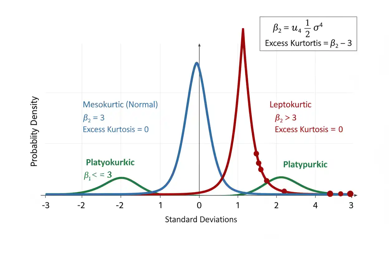
Kurtosis is a dimensionless statistical measure based on the fourth standardized moment of a distribution, describing how strongly probability or observed data are associated with large deviations from the mean relative to the distribution’s variance. For a population with finite fourth moment and positive variance, kurtosis is β₂ = μ₄/σ⁴, where μ₄ is the fourth central moment and σ⁴ is the square of the variance, while excess kurtosis subtracts the normal-distribution benchmark of 3 so that a normal distribution has excess kurtosis equal to zero. Because deviations are raised to the fourth power, observations far from the mean receive extremely large mathematical weight, making kurtosis particularly sensitive to tail behavior and extreme values. Positive excess kurtosis is conventionally called leptokurtic, zero excess kurtosis mesokurtic, and negative excess kurtosis platykurtic, although these labels should not be reduced to simplistic descriptions of whether a distribution has a sharp or flat peak. Kurtosis is fundamentally a fourth-moment measure, and much of its practical behavior is driven by the tails and the possibility of extreme observations rather than by the center of the distribution alone.
Within descriptive statistics and the broader Statistics & Probability framework, kurtosis is most informative when it is interpreted alongside measures of center, spread, skewness, and graphical distribution shape. A numerical kurtosis value can signal unusually strong tail influence, but it cannot by itself reveal whether extreme observations occur mainly on the left, the right, or both sides, nor can it show multimodality, gaps, or other structural features of the data.
What Is Kurtosis?
Kurtosis measures the fourth standardized moment of a distribution.
For a random variable X with population mean μ and standard deviation σ:
β₂ = E[(X − μ)⁴] / σ⁴
Because:
μ₄ = E[(X − μ)⁴]
the same formula can be written:
β₂ = μ₄/σ⁴
where:
- β₂ = population kurtosis
- μ₄ = fourth central moment
- σ = population standard deviation
- σ⁴ = variance squared
The fourth power causes large deviations from the mean to contribute disproportionately to the result.
That property is central to understanding kurtosis.
What Is Excess Kurtosis?
The normal distribution has kurtosis:
β₂ = 3
so excess kurtosis is defined as:
γ₂ = β₂ − 3
Therefore, a normal distribution has:
γ₂ = 0.
This adjusted form makes interpretation easier because zero becomes the normal benchmark.
When software reports “kurtosis,” it may provide either:
ordinary kurtosis β₂
or:
excess kurtosis γ₂.
The distinction must be checked before interpreting the number.
Kurtosis vs Excess Kurtosis
Suppose a distribution has:
β₂ = 5.
Its excess kurtosis is:
γ₂ = 5 − 3
= 2.
Both values describe the same distribution.
The difference is only the benchmark.
Ordinary kurtosis compares directly with:
3
while excess kurtosis compares directly with:
Therefore:
β₂ = 5
and:
γ₂ = 2
should not be interpreted as two different levels of tail behavior.
Why the Fourth Power Is Used
Variance is based on squared deviations:
(X − μ)².
Kurtosis uses:
(X − μ)⁴.
Suppose two observations are:
1 standard deviation
and:
4 standard deviations
from the mean.
Their squared standardized deviations are:
1² = 1
and:
4² = 16.
Their fourth powers are:
1⁴ = 1
and:
4⁴ = 256.
Thus, the four-standard-deviation observation contributes 256 times as much as the one-standard-deviation observation to the raw standardized fourth-power calculation.
Kurtosis is therefore highly responsive to extreme deviations.
Population Kurtosis Formula
The population fourth central moment is:
μ₄ = E[(X − μ)⁴]
For a finite population of N observations:
μ₄ = Σ(xᵢ − μ)⁴/N
Population variance is:
σ² = Σ(xᵢ − μ)²/N
Therefore:
σ⁴ = (σ²)²
and population kurtosis becomes:
β₂ = [Σ(xᵢ − μ)⁴/N] / σ⁴
or equivalently:
β₂ = μ₄/(μ₂)²
because:
μ₂ = σ².
Excess kurtosis is then:
γ₂ = β₂ − 3.
Simple Kurtosis Example
Consider the finite population:
1, 2, 3, 4, 5
The mean is:
μ = 3.
Deviations are:
−2, −1, 0, 1, 2.
Squared deviations are:
4, 1, 0, 1, 4.
Their mean is:
μ₂ = (4 + 1 + 0 + 1 + 4)/5
= 10/5
= 2.
Therefore:
σ² = 2.
Calculate the Fourth Central Moment
Raise each deviation to the fourth power:
(−2)⁴ = 16
(−1)⁴ = 1
0⁴ = 0
1⁴ = 1
2⁴ = 16
The total is:
Therefore:
μ₄ = 34/5
= 6.8.
Now calculate:
β₂ = μ₄/(μ₂)²
= 6.8/2²
= 6.8/4
= 1.7.
Thus, the population kurtosis is:
1.7.
Calculate Excess Kurtosis
Excess kurtosis is:
γ₂ = 1.7 − 3
= −1.3.
Therefore, this five-value population has:
Excess kurtosis = −1.3.
Relative to the normal-distribution benchmark, this is a negative excess-kurtosis example.
The term traditionally used is:
platykurtic.
The calculation does not mean the data must have a particular visually “flat” peak; it means their standardized fourth moment is below the normal benchmark.
Mesokurtic Distribution
A distribution with:
β₂ = 3
or:
γ₂ = 0
is called mesokurtic relative to the conventional normal benchmark.
The normal distribution is the standard example.
Mesokurtic does not mean that every feature of the distribution matches a normal distribution.
Two non-normal distributions can potentially have the same fourth standardized moment.
The term refers specifically to the kurtosis benchmark rather than complete equality of distribution shape.
Leptokurtic Distribution
A distribution with:
β₂ > 3
or:
γ₂ > 0
is called leptokurtic.
Positive excess kurtosis means the fourth standardized moment exceeds that of a normal distribution.
In practice, this often corresponds to a distribution in which extreme deviations exert substantial influence and tail behavior is more pronounced relative to the variance.
However, calling every leptokurtic distribution simply “more peaked” is misleading because kurtosis does not measure central peak height independently of the tails.
Platykurtic Distribution
A distribution with:
β₂ < 3
or:
γ₂ < 0
is called platykurtic.
Its fourth standardized moment lies below the normal benchmark.
For example, a continuous uniform distribution has population kurtosis:
β₂ = 9/5
= 1.8
and excess kurtosis:
γ₂ = 1.8 − 3
= −1.2.
The uniform distribution therefore provides a familiar theoretical example of negative excess kurtosis.
Kurtosis Is Not Simply Peakedness
Kurtosis is frequently described as measuring the “peakedness” of a distribution, but that description is incomplete and can be misleading.
The formula contains:
(X − μ)⁴
which gives enormous mathematical weight to observations far from the mean.
Consequently, two distributions can differ substantially in their central shapes while having similar kurtosis values, and a high-kurtosis distribution need not have the visually tallest central peak.
A better interpretation emphasizes:
tail extremity and large standardized deviations.
The center still contributes to the fourth moment, but extreme observations can dominate it.
Why Tails Matter So Much
Suppose most standardized deviations are around:
±1
but one observation lies:
6
standard deviations from the mean.
That observation contributes:
6⁴ = 1296
to the standardized fourth-power total.
An observation one standard deviation away contributes:
Thus, one extreme observation can contribute as much fourth-power weight as more than a thousand ordinary one-standard-deviation observations before averaging effects are considered.
This explains why sample kurtosis can change dramatically when even a small number of extreme observations enter or leave the data set.
Kurtosis and Outliers
Kurtosis is highly sensitive to outliers.
Consider a data set whose observations are mostly close together, then add one value far from the mean.
That new observation affects the kurtosis calculation in several ways:
- it changes the mean;
- it changes the variance;
- most importantly, its fourth-power deviation can become enormous.
Therefore, a large sample kurtosis can serve as a warning that extreme observations deserve examination.
It does not prove those observations are errors.
They may represent genuine rare events or heavy-tailed population behavior.
Extreme-Value Example
Consider the population:
0, 0, 0, 0, 0, 0, 0, 0, 0, 10
The mean is:
μ = 1.
Nine observations have deviation:
−1
and one observation has deviation:
The population second central moment is:
μ₂ = [9(1²) + 9²]/10
= (9 + 81)/10
= 9.
Therefore:
σ² = 9.
Fourth Moment of the Extreme-Value Example
The fourth central moment is:
μ₄ = [9(1⁴) + 9⁴]/10
Since:
9⁴ = 6561
we obtain:
μ₄ = (9 + 6561)/10
= 657.
Therefore:
β₂ = 657/9²
= 657/81
≈ 8.111.
Excess kurtosis is:
γ₂ ≈ 8.111 − 3
≈ 5.111.
One distant observation produces strongly positive excess kurtosis.
Interpreting the Extreme Example
The result:
γ₂ ≈ 5.111
does not mean only that the distribution has a sharp center.
The defining numerical feature is that one observation lies far from the mean relative to the overall variance and contributes:
6561
to the fourth-power deviation total.
This example demonstrates why high kurtosis is closely associated with sensitivity to extreme deviations.
Graphical examination is essential because the same one-number result cannot show exactly which observations created it.
Kurtosis and Histograms
A histogram provides distributional information that kurtosis alone cannot preserve.
For example, it can reveal whether a large kurtosis value arises alongside:
- two long tails;
- one extreme upper tail;
- one isolated observation;
- several clusters;
- a mixture of populations.
Kurtosis quantifies fourth-moment behavior.
The graph shows where observations actually occur.
Using both is more informative than interpreting the numerical statistic in isolation.
Kurtosis and Skewness
Skewness and kurtosis describe different standardized moments.
Skewness is based on a third power:
E[(X − μ)³]/σ³
and measures directional asymmetry.
Kurtosis uses a fourth power:
E[(X − μ)⁴]/σ⁴.
Because fourth powers are always nonnegative, kurtosis does not retain the direction of an extreme observation.
A very large negative deviation and a similarly large positive deviation contribute equally after being raised to the fourth power.
Why Kurtosis Does Not Show Tail Direction
Suppose standardized deviations include:
−5
and:
+5.
Their fourth powers are:
(−5)⁴ = 625
and:
(+5)⁴ = 625.
Therefore, kurtosis treats these deviations equally.
Skewness does not:
(−5)³ = −125
(+5)³ = 125.
Thus, skewness indicates directional imbalance, while kurtosis emphasizes magnitude of extreme standardized deviations regardless of direction.
Both can be useful when describing asymmetric heavy-tailed data.
Kurtosis and Variance
Variance is:
μ₂ = E[(X − μ)²].
Kurtosis standardizes the fourth central moment by:
μ₂².
Therefore:
β₂ = μ₄/μ₂².
This standardization removes measurement units.
If X is measured in meters, μ₄ has units:
meters⁴
while μ₂² also has:
meters⁴.
The units cancel.
Kurtosis is therefore dimensionless and can describe shape without depending on the original unit scale.
Scale Invariance
Suppose:
Y = aX + b
with:
a ≠ 0.
The fourth central moment transforms as:
μ₄,Y = a⁴μ₄,X
while variance becomes:
σ²_Y = a²σ²_X.
Therefore:
σ⁴_Y = a⁴σ⁴_X.
The scale factors cancel:
β₂,Y = a⁴μ₄,X / a⁴σ⁴_X
= β₂,X.
Thus, kurtosis does not change when a variable is shifted or multiplied by a nonzero constant.
Unit Conversion Example
Suppose a height distribution is measured in:
meters
and then converted to:
centimeters.
Every deviation is multiplied by:
The fourth central moment is multiplied by:
100⁴,
while σ⁴ is also multiplied by:
100⁴.
Their ratio remains unchanged.
Therefore, kurtosis is identical whether the heights are reported in meters, centimeters, or another linearly related unit.
Translation Invariance
Adding a constant also leaves kurtosis unchanged.
If:
Y = X + 100
then both variables have the same centered deviations because:
Y − μY = X − μX.
Therefore:
μ₂,Y = μ₂,X
and:
μ₄,Y = μ₄,X.
Kurtosis does not depend on the arbitrary location of zero on the measurement scale.
It depends on standardized shape around the mean.
Sample Kurtosis
When population moments are unknown, kurtosis is estimated from sample observations.
Define sample central moments using denominator n:
m₂ = Σ(xᵢ − x̄)²/n
m₄ = Σ(xᵢ − x̄)⁴/n.
A simple moment-based sample kurtosis is:
b₂ = m₄/m₂².
A corresponding sample excess kurtosis is:
g₂ = m₄/m₂² − 3.
This estimator is straightforward but is biased for population excess kurtosis in finite samples.
Different statistical programs can therefore use corrected formulas.
Bias-Corrected Sample Excess Kurtosis
A commonly used adjusted Fisher–Pearson sample excess kurtosis is:
G₂ = [(n − 1)/((n − 2)(n − 3))] × [(n + 1)g₂ + 6]
for:
n > 3.
Here:
g₂ = m₄/m₂² − 3.
This correction reduces finite-sample bias under common assumptions.
The important practical lesson is that “sample kurtosis” is not represented by one universally implemented finite-sample formula.
Software definitions must be checked before comparing values.
Sample Formula Example
Return to the sample:
1, 2, 3, 4, 5.
Using the moment calculation:
m₂ = 2
and:
m₄ = 6.8.
Therefore:
g₂ = 6.8/2² − 3
= 1.7 − 3
= −1.3.
For:
n = 5,
the adjusted estimator is:
G₂ = [4/(3×2)] × [6(−1.3) + 6]
= (4/6)(−1.8)
= −1.2.
Thus, two legitimate sample formulas give:
−1.3
and:
−1.2.
Why Software Can Report Different Kurtosis Values
Suppose the same sample is entered into two programs.
One program may return ordinary kurtosis:
b₂.
Another may return excess kurtosis:
g₂.
A third may apply finite-sample bias correction:
G₂.
Consequently, values can differ by:
exactly 3
or by a smaller bias-correction adjustment.
Before concluding that one program is wrong, determine:
- whether it reports excess or ordinary kurtosis;
- which sample estimator it uses.
The definition matters as much as the input data.
Population vs Sample Kurtosis
For a complete finite population, the moment ratio:
β₂ = μ₄/σ⁴
describes that defined population directly.
For a sample drawn from a larger population, a calculated kurtosis is a statistic and varies from sample to sample.
A sample of:
n = 20
can produce a very high kurtosis because one unusual observation happened to be selected, even when the population kurtosis is much more moderate.
Sampling variability can therefore be substantial, particularly for fourth-moment statistics.
Why Kurtosis Is Unstable in Small Samples
The fourth power magnifies the influence of the most extreme sampled observations.
Small samples contain relatively little information about rare tail events, yet one such event can dominate the statistic.
Therefore, sample kurtosis can fluctuate considerably between repeated small samples from the same population.
A large numerical difference between two small-sample kurtosis values does not automatically indicate that the underlying populations have dramatically different tail behavior.
Sample size should always be considered.
Normal Distribution Kurtosis
For a normal distribution:
β₂ = 3.
Therefore:
γ₂ = 0.
This benchmark is the reason excess kurtosis subtracts three.
It does not mean that every sample from a normal population will have sample excess kurtosis exactly zero.
Finite random samples naturally produce:
positive
or:
negative
sample estimates around the population value.
The amount of sampling variability can be substantial when n is small.
Uniform Distribution Kurtosis
For a continuous uniform distribution over a finite interval:
β₂ = 9/5
= 1.8.
Therefore:
γ₂ = −1.2.
This is a standard platykurtic example relative to the normal benchmark.
The bounded support prevents arbitrarily large tail observations.
That structural difference contributes to its smaller standardized fourth moment.
Student’s t Distribution and Kurtosis
Student’s t distributions provide a useful illustration of heavy-tail behavior.
For degrees of freedom:
ν > 4,
the excess kurtosis is:
γ₂ = 6/(ν − 4).
Therefore, with:
ν = 10,
we obtain:
γ₂ = 6/(10 − 4)
= 1.
The ordinary kurtosis is:
β₂ = 4.
As ν increases, the t distribution approaches the normal distribution and excess kurtosis approaches zero.
When Kurtosis Does Not Exist
Not every probability distribution has a finite fourth moment.
For a Student’s t distribution with:
ν ≤ 4,
the fourth moment is not finite.
Therefore, population kurtosis is not finite in the ordinary fourth-moment sense.
This is an important limitation.
A finite data sample always contains finite observed numbers and can produce a numerical sample kurtosis, but that does not imply the theoretical population distribution has a finite kurtosis parameter.
Existence of Mean, Variance, and Kurtosis
Different moments require different levels of tail decay.
A distribution can have:
a finite mean
but:
infinite variance.
Another can have:
finite variance
but:
infinite fourth moment.
In the latter case, ordinary variance exists but kurtosis does not.
This hierarchy illustrates why kurtosis is especially demanding of tail behavior: fourth moments are more sensitive to extreme values than second moments.
Kurtosis and Heavy Tails
Positive excess kurtosis is often associated with distributions that generate extreme observations more readily than a normal distribution with comparable variance.
However, “heavier tails” should be used carefully because tail comparisons can be defined in several mathematical ways.
Kurtosis is a global fourth-moment quantity rather than a direct measurement of one particular tail probability.
Two distributions can have similar kurtosis yet differ in their detailed extreme-event probabilities.
Thus, kurtosis is a useful summary, not a complete tail model.
High Kurtosis Does Not Identify the Cause
Suppose sample excess kurtosis is:
Several very different data-generating patterns could produce that result.
The data might contain:
one extremely distant observation,
several moderately extreme observations, or a genuinely heavy-tailed continuous population.
It might also combine distinct subgroups.
The numerical statistic cannot distinguish these mechanisms by itself.
That is why graphical examination and domain context should accompany unusually large kurtosis values.
Kurtosis and the Median
The median is a rank-based measure of center and is comparatively resistant to extreme observations.
Kurtosis behaves very differently because fourth powers deliberately magnify extreme deviations.
Suppose one upper observation moves from:
20
to:
20,000.
The median of a sufficiently large ordered data set might remain exactly unchanged, while sample kurtosis can increase enormously.
The two statistics therefore answer almost opposite descriptive questions: the median locates a resistant center, whereas kurtosis emphasizes extreme standardized departures from the center.
Kurtosis and Geometric Mean
The geometric mean provides a multiplicative center for suitable positive observations, whereas kurtosis describes fourth-moment tail behavior after centering around the arithmetic mean.
A data set can have a useful geometric mean and extremely high kurtosis at the same time.
For example, positive lognormal-type data can display strong right tails while retaining a meaningful multiplicative center.
A measure of center does not replace a measure of distribution shape.
Kurtosis and Harmonic Mean
The harmonic mean is especially sensitive to very small positive observations because it operates on reciprocals, whereas kurtosis is sensitive to observations that lie far from the arithmetic mean in either direction.
Thus, the two measures can react to different parts of the same data set.
One extremely small positive rate may dominate a harmonic mean even if its standardized distance from the mean is not the most extreme feature, while one enormous upper observation can heavily influence kurtosis.
Understanding the transformation behind each statistic explains these differences.
Kurtosis and Margin of Error
A margin of error describes uncertainty around an estimated population parameter under a particular inferential procedure.
Kurtosis instead describes fourth-moment distribution shape.
However, heavy-tailed data can indirectly affect inferential precision because extreme observations can increase variability and make normal approximations less reliable in small samples.
A kurtosis value is not itself a margin of error and should not be interpreted as an uncertainty bound.
The two concepts operate at different statistical levels.
Can Kurtosis Be Negative?
Ordinary kurtosis:
β₂ = μ₄/σ⁴
cannot be negative because both numerator and denominator are nonnegative when variance is positive.
In fact, ordinary kurtosis has a lower theoretical bound of at least:
1
for non-degenerate distributions under the standard moment definition.
Excess kurtosis:
γ₂ = β₂ − 3
can be negative.
Therefore, a reported value such as:
−1.2
must represent excess kurtosis rather than ordinary kurtosis.
This is another useful clue when interpreting software output.
Minimum Possible Kurtosis
For a non-degenerate random variable with finite moments:
β₂ ≥ 1.
One way to see this is through the relationship between second and fourth moments.
Therefore:
γ₂ ≥ −2.
The lower bound for excess kurtosis is:
−2.
A two-point distribution with equal probability at symmetric endpoints achieves this limiting value.
Consequently, an ordinary excess-kurtosis calculation below −2 indicates a formula or implementation issue.
Can Kurtosis Be Very Large?
Yes.
There is no finite universal upper bound on kurtosis.
A distribution can place very small probability on observations extremely far from its center, producing an enormous fourth moment relative to its variance squared.
Likewise, a finite sample can produce a very large sample kurtosis when one or a few observations lie far from the rest.
High values should therefore prompt inspection of the tails and raw observations.
Can Kurtosis Equal 3 Without Normality?
Yes.
Kurtosis:
β₂ = 3
does not imply the distribution is normal.
It only says the fourth standardized moment equals the normal benchmark.
Different distributions can share the same first several moments while having different shapes.
Therefore:
excess kurtosis = 0
means mesokurtic relative to the normal reference, not “proven normal.”
Normality requires far more information than one fourth-moment statistic.
Can a Symmetric Distribution Have High Kurtosis?
Yes.
Symmetry concerns directional balance around a center.
Kurtosis concerns the magnitude of fourth-power deviations.
A symmetric distribution can have heavy tails on both sides and therefore high positive excess kurtosis.
Student’s t distributions are classic examples: they are symmetric but can have much heavier tails than a normal distribution.
Thus:
symmetry ≠ low kurtosis.
Can a Skewed Distribution Have Low Kurtosis?
Yes.
Skewness and kurtosis are separate moment characteristics.
A distribution can be asymmetric yet have a standardized fourth moment below the normal benchmark.
Likewise, a symmetric distribution can have high positive excess kurtosis.
The values should therefore be interpreted independently and then considered together as part of a broader distributional description.
Kurtosis and Outlier Detection
Kurtosis can indicate that extreme observations strongly affect the distribution, but it is not a direct outlier-identification rule.
A large kurtosis value does not tell which specific observation should be classified as an outlier.
Methods based on:
IQR fences,
standardized residuals, robust distances, or domain-specific thresholds may identify individual observations more directly.
Kurtosis answers a population- or sample-level shape question rather than assigning labels to individual records.
Effect of Removing an Extreme Observation
Suppose a sample has very high kurtosis because of one distant observation.
Removing that observation can cause the estimate to fall sharply.
This sensitivity does not automatically justify removal.
The correct question is whether the observation is:
erroneous,
irrelevant to the target population, or genuinely part of the process being studied.
If it is genuine, removing it merely to make kurtosis look more normal discards real distributional information.
Effect of Measurement Errors
A decimal-point error can produce enormous fourth-power consequences.
Suppose a value intended as:
10
is recorded as:
Its deviation from the mean can become orders of magnitude larger than all others.
Raising that deviation to the fourth power can dominate the sample kurtosis.
Extremely large kurtosis should therefore sometimes trigger data-quality checks, especially when the observed value is implausible in context.
Kurtosis for Grouped Data
If only grouped frequency intervals are available, kurtosis can be approximated using class midpoints.
Let:
mᵢ = midpoint of class i
and:
fᵢ = class frequency.
An approximate grouped mean is calculated first, followed by approximate second and fourth central moments:
m₂ ≈ Σfᵢ(mᵢ − x̄)²/n
m₄ ≈ Σfᵢ(mᵢ − x̄)⁴/n.
Then:
b₂ ≈ m₄/m₂².
The result is approximate because every observation within each class is treated as though it lies at the midpoint.
Frequency Distribution Formula
For discrete observations summarized by ordinary frequencies, the moment calculation can be performed exactly when the distinct values themselves are known.
If xᵢ occurs fᵢ times:
n = Σfᵢ
x̄ = Σfᵢxᵢ/n
Then:
m₂ = Σfᵢ(xᵢ − x̄)²/n
and:
m₄ = Σfᵢ(xᵢ − x̄)⁴/n.
Therefore:
b₂ = m₄/m₂²
and:
g₂ = b₂ − 3.
Frequency weights simply avoid writing repeated observations individually.
Kurtosis and Standardization
Define standardized values:
zᵢ = (xᵢ − μ)/σ
for a population.
Then:
β₂ = E(z⁴).
Thus, kurtosis can be interpreted as the expected fourth power of standardized distance from the mean.
A standardized observation of:
z = 2
contributes:
2⁴ = 16.
A standardized observation of:
z = 5
contributes:
5⁴ = 625.
This standardized formulation makes the extreme-value sensitivity particularly clear.
Why Variance Is Squared in the Denominator
The fourth central moment has units raised to the fourth power.
Variance has units squared.
Therefore:
Variance²
has fourth-power units.
Dividing:
μ₄/σ⁴
removes units and creates a scale-free measure.
Without this standardization, the fourth central moment of measurements recorded in centimeters would be enormously larger numerically than the same data recorded in meters.
Kurtosis avoids that unit dependence.
Kurtosis and Mixture Distributions
Combining groups can materially alter kurtosis.
Suppose two populations individually have moderate tail behavior but very different centers.
Combining them can create:
- a broad distribution;
- multiple modes;
- unusual standardized deviations.
The resulting kurtosis may differ sharply from either subgroup’s value.
Therefore, a high or low overall kurtosis can sometimes reflect unmodeled population heterogeneity rather than one homogeneous distribution.
Group structure should be examined where relevant.
Kurtosis and Transformations
Linear transformations do not change kurtosis, but nonlinear transformations can.
For a positive variable:
Y = ln(X)
can substantially reduce a long right tail.
The kurtosis of:
ln(X)
can therefore differ dramatically from the kurtosis of X.
This is not a contradiction.
The logarithm changes the distribution’s relative distances, especially among large observations.
Kurtosis should always be interpreted on the scale on which it was calculated.
Raw-Scale vs Log-Scale Kurtosis
Suppose positive measurements span:
1 to 100,000.
On the raw scale, upper observations can dominate fourth-power deviations.
Taking logarithms compresses those large ratios.
The resulting log-scale distribution can have much lower sample kurtosis.
If the underlying scientific process is multiplicative, the log-scale description may be substantively meaningful.
However, raw-scale and log-scale kurtosis answer different questions and should not be compared as though they described identical geometry.
Sample Size and Extreme Events
As sample size increases, the opportunity to observe rare tail events also increases.
A large sample can therefore include observations more extreme than anything seen in a small sample.
This does not imply the large sample is worse behaved.
It may simply reveal more of the true population tails.
Consequently, comparing raw maximum values or sample kurtosis across dramatically different sample sizes requires care.
Kurtosis and Risk
In applications involving losses, returns, engineering loads, or other extreme-event concerns, kurtosis is sometimes used as an indicator that tail observations deserve more attention than a normal model would suggest.
However, kurtosis is not a complete risk measure.
It does not distinguish upper and lower tails and does not directly report probabilities such as:
P(X < threshold)
or:
P(X > threshold).
When specific tail events matter, quantiles, tail probabilities, expected shortfall, or domain-specific extreme-value methods can provide more targeted information.
Kurtosis and Practical Interpretation
A statistically large kurtosis value does not automatically imply a practical problem.
If extreme observations are genuine and expected, high kurtosis may simply describe the process correctly.
Conversely, a moderate kurtosis value does not guarantee that no important extreme event exists.
A rare but consequential observation can matter operationally even if the overall fourth-moment estimate is not dramatic.
Statistical summaries should always be connected back to the consequences and context of the data.
Common Kurtosis Mistakes
A common mistake is interpreting kurtosis purely as peak height. Because fourth-power deviations strongly weight extreme observations, tail behavior is central to the statistic.
Another error is comparing a reported excess kurtosis directly with ordinary-kurtosis benchmark 3. Excess kurtosis should be compared with:
Ordinary kurtosis should be compared with:
Analysts also sometimes compare software outputs without checking whether the programs use biased or bias-corrected sample estimators.
Another mistake is assuming:
excess kurtosis = 0
proves normality.
It does not.
Removing extreme observations solely because they raise sample kurtosis is also inappropriate unless there is an independent reason to exclude them.
Finally, a very large finite sample statistic does not guarantee that a theoretical population fourth moment exists.
How to Calculate Kurtosis Step by Step
Begin with a numerical data set having nonzero variance.
Calculate the mean:
x̄ = Σxᵢ/n.
Then find each deviation:
xᵢ − x̄.
Calculate the second central moment:
m₂ = Σ(xᵢ − x̄)²/n.
Next calculate the fourth central moment:
m₄ = Σ(xᵢ − x̄)⁴/n.
The moment-based sample kurtosis is:
b₂ = m₄/m₂².
Excess kurtosis is:
g₂ = b₂ − 3.
If finite-sample bias correction is required, apply the specific corrected estimator appropriate to the software, method, and inferential context.
Full Worked Kurtosis Example
Consider:
1, 2, 3, 4, 5
Step 1: Mean
x̄ = (1 + 2 + 3 + 4 + 5)/5
= 15/5
= 3
Step 2: Deviations
−2, −1, 0, 1, 2
Step 3: Squared Deviations
4, 1, 0, 1, 4
Their sum is:
Therefore:
m₂ = 10/5
= 2
Step 4: Fourth-Power Deviations
16, 1, 0, 1, 16
Their sum is:
Therefore:
m₄ = 34/5
= 6.8
Step 5: Moment Kurtosis
b₂ = 6.8/2²
= 1.7
Step 6: Excess Kurtosis
g₂ = 1.7 − 3
= −1.3
Under this moment convention:
Kurtosis = 1.7
Excess kurtosis = −1.3.
Bias-Correct the Worked Sample
Because:
n = 5,
a commonly used corrected excess estimator gives:
G₂ = [(n − 1)/((n − 2)(n − 3))] × [(n + 1)g₂ + 6]
Substitute:
n = 5
and:
g₂ = −1.3.
Then:
G₂ = [4/(3×2)] × [6(−1.3) + 6]
= 4/6 × (−7.8 + 6)
= 4/6 × (−1.8)
= −1.2.
Therefore, corrected sample excess kurtosis is:
−1.2.
The difference illustrates why the estimator definition should accompany precise sample-kurtosis calculations.
Comparing a Data Set Before and After an Extreme Observation
Suppose a compact sample has relatively modest fourth-power deviations.
Now replace one ordinary upper value with an observation several standard deviations above the center.
The fourth central moment can increase far more rapidly than the variance because:
deviation⁴
grows faster than:
deviation².
Consequently, the kurtosis ratio can rise sharply.
This mathematical behavior explains why kurtosis is often useful for detecting distributions in which unusually distant observations play a disproportionate role.
How to Interpret Kurtosis in Practice
A practical interpretation should begin by identifying which convention is being reported.
For example:
“Excess kurtosis was 2.4.”
This immediately indicates a value:
2.4 above the normal benchmark.
Next examine the distribution graphically to determine whether the positive result appears to arise from:
- broad heavy tails;
- isolated extremes;
- asymmetry;
- mixed subgroups.
Finally, consider sample size and data quality before assigning substantive meaning.
Kurtosis is most valuable as part of a coordinated distributional analysis rather than as a standalone label.
How to Report Kurtosis
A clear report might state:
“The sample excess kurtosis was 2.1 using the bias-corrected Fisher–Pearson estimator, indicating stronger fourth-moment tail influence than the normal-distribution benchmark.”
For negative kurtosis:
“The excess kurtosis was −1.0, below the normal benchmark of zero.”
When sample size is small or extreme observations dominate the estimate, note that the statistic is sensitive to those observations.
If software is used, specifying whether the result is ordinary or excess kurtosis can prevent a three-unit interpretation error.
Frequently Asked Questions About Kurtosis
What is kurtosis?
Kurtosis is the fourth standardized moment of a distribution, measuring the influence of large standardized deviations from the mean.
What is the population kurtosis formula?
β₂ = μ₄/σ⁴
What is another form of the formula?
β₂ = E[(X − μ)⁴]/σ⁴
What is excess kurtosis?
γ₂ = β₂ − 3
Why subtract 3?
Because the normal distribution has ordinary kurtosis equal to 3.
What is normal-distribution excess kurtosis?
0
What is normal-distribution ordinary kurtosis?
3
What does positive excess kurtosis mean?
It means the standardized fourth moment is greater than the normal benchmark.
What is a leptokurtic distribution?
A distribution with:
Excess kurtosis > 0.
What is a mesokurtic distribution?
A distribution with:
Excess kurtosis = 0
relative to the normal benchmark.
What is a platykurtic distribution?
A distribution with:
Excess kurtosis < 0.
Does kurtosis measure peak height?
Not directly. It is a fourth-moment measure strongly influenced by extreme deviations and tails.
Why are outliers important for kurtosis?
Because deviations are raised to the fourth power, so distant observations receive very large weights.
Is kurtosis sensitive to outliers?
Yes, extremely.
Does kurtosis show whether an extreme value is above or below the mean?
No. Fourth powers eliminate the sign of deviations.
Which statistic captures directional asymmetry?
Skewness.
Can a symmetric distribution have high kurtosis?
Yes.
Can a skewed distribution have negative excess kurtosis?
Yes.
Does zero excess kurtosis prove normality?
No.
Can non-normal distributions have kurtosis of 3?
Yes.
Is kurtosis affected by measurement units?
No. It is standardized and dimensionless.
Does converting meters to centimeters change kurtosis?
No.
Does adding a constant to every observation change kurtosis?
No.
Does multiplying every observation by a constant change kurtosis?
Not when multiplied by a nonzero constant under the standard definition.
Can ordinary kurtosis be negative?
No.
Can excess kurtosis be negative?
Yes.
What is the lower bound of ordinary kurtosis?
For a non-degenerate distribution under the standard moment definition:
β₂ ≥ 1.
What is the lower bound of excess kurtosis?
γ₂ ≥ −2.
Does kurtosis have an upper limit?
No finite universal upper limit exists.
What is sample excess kurtosis?
A basic moment form is:
g₂ = m₄/m₂² − 3.
Why can sample kurtosis formulas differ?
Different estimators use different finite-sample bias corrections and may report ordinary or excess kurtosis.
What is a common corrected sample excess formula?
G₂ = [(n − 1)/((n − 2)(n − 3))][(n + 1)g₂ + 6]
for n > 3.
Why is sample kurtosis unstable for small n?
Rare extreme observations have enormous fourth-power influence, while small samples contain limited information about population tails.
What is the kurtosis of a normal distribution?
3
or excess:
What is the kurtosis of a continuous uniform distribution?
1.8
with excess:
−1.2.
What is the excess kurtosis of a Student’s t distribution?
For:
ν > 4
it is:
6/(ν − 4).
Does every distribution have finite kurtosis?
No.
Can variance exist while kurtosis does not?
Yes. A distribution can have a finite second moment but an infinite fourth moment.
Can a finite sample have numerical kurtosis even when population kurtosis is infinite?
Yes. A finite observed data set contains finite values, but the theoretical population fourth moment may still diverge.
Is high kurtosis the same as having many outliers?
Not exactly. A few extremely distant observations can generate high kurtosis, as can broader heavy-tail behavior.
Can kurtosis identify which observations are outliers?
No. It is a distribution-level summary.
Should observations be deleted because they increase kurtosis?
No. They should be removed only when there is an independent reason, such as verified data error or irrelevance to the target population.
Can grouped data be used to estimate kurtosis?
Yes, approximately, by using class midpoints and frequencies.
Is grouped-data kurtosis exact?
Usually not if the original observations are unavailable.
How does kurtosis differ from variance?
Variance measures average squared deviation, while kurtosis uses the fourth moment standardized by variance squared and is far more sensitive to extreme deviations.
How does kurtosis differ from skewness?
Skewness measures directional asymmetry using the third standardized moment; kurtosis uses the fourth standardized moment and does not retain direction.
How should kurtosis be interpreted with a histogram?
Use the numerical value to assess fourth-moment extremity and the graph to identify where tail observations, clusters, or asymmetry occur.
What is the biggest misconception about kurtosis?
The biggest misconception is that it is simply a measure of how pointed or flat a distribution’s central peak looks. Its fourth-power definition makes extreme standardized deviations and tail behavior central to its interpretation.
What is the most important rule when using kurtosis?
Always identify whether the reported value is ordinary or excess kurtosis, check the sample estimator being used, inspect the actual distribution for extreme observations and tail structure, and avoid treating one fourth-moment statistic as a complete description of distribution shape.




