


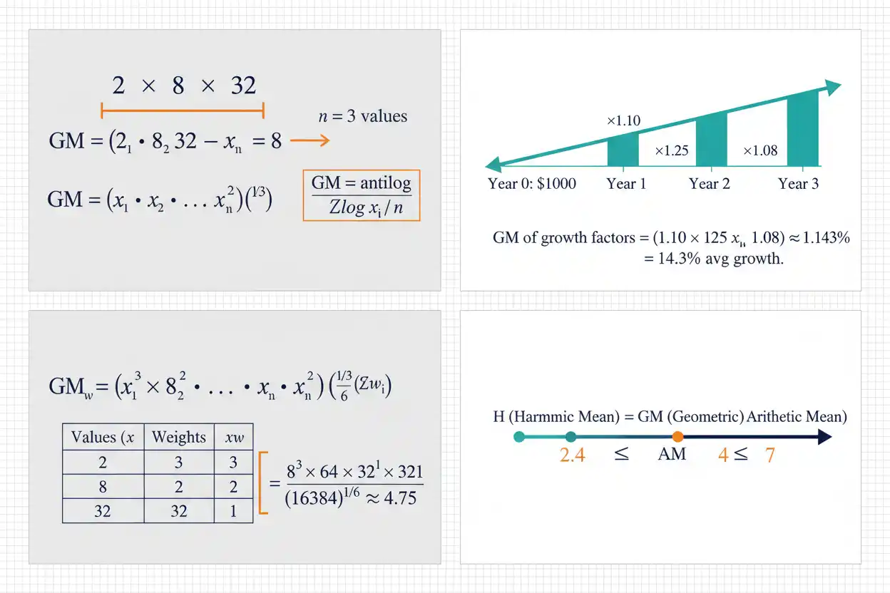
The geometric mean is a measure of central tendency calculated by multiplying positive values together and taking the nth root of the resulting product, making it particularly useful when observations combine multiplicatively rather than additively. For n positive observations x₁, x₂, …, xₙ, the geometric mean is GM = (x₁x₂…xₙ)^(1/n), which differs fundamentally from the arithmetic mean because it balances proportional changes and ratios rather than equal absolute differences. This makes the geometric mean especially valuable for compound growth factors, repeated percentage changes, index relatives, normalized ratios, and other situations in which one period or observation acts on the result of another. A return of +50% followed by −50%, for example, does not average to zero in compounded-value terms because multiplication by 1.5 and then 0.5 leaves only 75% of the original value; the geometric mean correctly captures that multiplicative outcome. The geometric mean is also less dominated by very large positive observations than the arithmetic mean, although it requires careful treatment of zero and negative values and should not be used merely because a data set is skewed.
The geometric mean belongs to the broader family of averages within descriptive statistics and Statistics & Probability. It is especially important when the data-generating structure is multiplicative, while the related harmonic mean is more naturally suited to selected rate and reciprocal problems and the arithmetic mean remains the standard choice for ordinary additive quantities.
What Is the Geometric Mean?
The geometric mean is the nth root of the product of n positive observations.
For:
x₁, x₂, …, xₙ
the formula is:
GM = (x₁x₂…xₙ)^(1/n)
Using product notation:
GM = (Πxᵢ)^(1/n)
where:
- GM = geometric mean
- xᵢ = individual positive observation
- n = number of observations
- Π = product of all observations
For two values:
GM = √(x₁x₂)
For three:
GM = ∛(x₁x₂x₃)
The geometric mean therefore depends on multiplication and roots rather than summation and division.
Simple Geometric Mean Example
Find the geometric mean of:
2 and 8
Multiply:
2 × 8 = 16
There are:
n = 2
observations, so take the square root:
GM = √16
GM = 4
Therefore:
Geometric mean = 4
The arithmetic mean of the same values is:
(2 + 8)/2 = 5
so the two averages are not generally equal.
Geometric Mean of Three Values
Consider:
4, 16, 64
Multiply:
4 × 16 × 64
= 4096
There are three observations, so:
GM = ∛4096
GM = 16
Therefore:
Geometric mean = 16
This example is particularly intuitive because the values form a multiplicative progression:
4 → 16 → 64
where each step multiplies by:
The middle value 16 is therefore the natural multiplicative center.
Why the Geometric Mean Is Different From the Arithmetic Mean
The arithmetic mean balances values according to additive distance.
The geometric mean balances them according to multiplicative proportion.
For:
2 and 8
the arithmetic mean is:
5
because:
5 − 2 = 3
and:
8 − 5 = 3.
The geometric mean is:
4
because the proportional relationships are balanced:
4/2 = 2
and:
8/4 = 2.
Thus, 4 sits halfway between 2 and 8 on a multiplicative scale.
This distinction is the central reason geometric mean is useful for ratios and compounding.
Geometric Mean Formula for Two Numbers
For two positive values a and b:
GM = √(ab)
Suppose:
a = 9
b = 16
Then:
GM = √(9 × 16)
= √144
= 12
The proportional ratios are:
12/9 = 4/3
and:
16/12 = 4/3.
The geometric mean therefore divides the multiplicative distance between the two values equally.
Geometric Mean Formula for Three Numbers
For three positive observations:
GM = ∛(abc)
Suppose:
1, 8, 27
Then:
GM = ∛(1 × 8 × 27)
= ∛216
= 6
Therefore:
GM = 6
The result does not need to be one of the original observations.
Like other measures of center, it summarizes the data rather than necessarily identifying an observed value.
General Geometric Mean Formula
For n positive values:
GM = (x₁x₂…xₙ)^(1/n)
The same formula can be expressed logarithmically as:
ln(GM) = [Σln(xᵢ)]/n
and therefore:
GM = exp{[Σln(xᵢ)]/n}
This logarithmic form is mathematically equivalent when every xᵢ is positive.
It is especially useful for large data sets because directly multiplying many large or very small values can cause numerical overflow or underflow in software.
Why Logarithms Work
Start with:
GM = (Πxᵢ)^(1/n)
Take natural logarithms:
ln(GM) = ln[(Πxᵢ)^(1/n)]
Use the power rule:
ln(GM) = (1/n)ln(Πxᵢ)
The logarithm of a product is the sum of logarithms:
ln(GM) = (1/n)Σln(xᵢ)
Therefore:
GM = exp[(1/n)Σln(xᵢ)]
This shows that the geometric mean is the arithmetic mean on the logarithmic scale transformed back to the original scale.
Geometric Mean as the Mean of Logarithms
For positive data, the calculation can be understood in three steps.
First transform each observation:
yᵢ = ln(xᵢ)
Then calculate the arithmetic mean of the logarithms:
ȳ = Σln(xᵢ)/n
Finally convert back:
GM = e^ȳ
This perspective explains several important properties of the geometric mean, including its suitability for multiplicative data and its invariance to proportional scaling.
It also shows why zero and negative observations create difficulties: ordinary real logarithms are not defined for them.
Geometric Mean and Growth Rates
One of the most important uses of the geometric mean is averaging compounded growth.
Suppose a quantity changes over three periods by:
+5%
+10%
−5%
Convert each percentage into a growth factor:
1.05
1.10
0.95
The geometric mean growth factor is:
GM = (1.05 × 1.10 × 0.95)^(1/3)
The product is:
1.09725
Therefore:
GM ≈ 1.03142
The equivalent compound average growth rate is:
1.03142 − 1
≈ 0.03142
or approximately:
3.14%
per period.
Why You Must Use Growth Factors
Percentage changes should not normally be inserted directly into the ordinary geometric-mean formula as signed percentages.
A decline of:
5%
corresponds to multiplication by:
0.95
not multiplication by:
−0.05.
Likewise, growth of:
20%
corresponds to:
1.20.
The correct procedure is:
Growth factor = 1 + decimal growth rate
Then calculate the geometric mean of the positive factors.
Finally subtract 1 to convert the average factor back into an average compound rate.
Geometric Mean of Returns Example
Suppose an investment has annual returns:
+20%
−10%
+15%
The growth factors are:
1.20
0.90
1.15
Their product is:
1.20 × 0.90 × 1.15
= 1.242
The geometric mean factor is:
GM = 1.242^(1/3)
≈ 1.0750
Therefore, the compound average return is approximately:
7.50%
per period.
The arithmetic mean return would be:
(20% − 10% + 15%)/3
= 8.33%
which is higher because it does not account for compounding drag.
+50% Followed by −50%
This classic example shows why arithmetic averaging can fail for compounded changes.
Start with:
100
After a:
+50%
increase:
100 × 1.50 = 150
Then apply:
−50%
150 × 0.50 = 75
The ending value is:
75
which represents a total loss of:
25%.
The arithmetic average of the two returns is:
(50% − 50%)/2
= 0%
but zero is not the compound average rate.
Geometric Mean for the +50% and −50% Example
The growth factors are:
1.50
and:
0.50
The average compound factor is:
GM = √(1.50 × 0.50)
= √0.75
≈ 0.8660
Convert back to a growth rate:
0.8660 − 1
= −0.1340
Therefore, the compound average rate is approximately:
−13.40%
per period.
Applying this same rate for two periods gives approximately the same total factor:
0.8660² ≈ 0.75.
Compound Annual Growth Rate
The geometric mean is closely related to compound annual growth rate.
If an initial value V₀ becomes Vₙ after n compounding periods:
Vₙ = V₀(1 + r)ⁿ
Solve for r:
1 + r = (Vₙ/V₀)^(1/n)
Therefore:
r = (Vₙ/V₀)^(1/n) − 1
This is the same multiplicative logic as the geometric mean.
The result is the constant per-period rate that would produce the same start-to-finish growth.
CAGR Example
Suppose a value grows from:
100
to:
172.8
over:
3 periods.
Then:
Growth factor = 172.8/100
= 1.728
Therefore:
1 + r = 1.728^(1/3)
= 1.20
so:
r = 0.20
or:
20%
per period.
A constant 20% compound rate produces:
100 × 1.2³
= 172.8.
Geometric Mean and Multiplicative Sequences
For a geometric progression:
a, ar, ar², …, ar^(n−1)
the geometric mean reflects the multiplicative center of the sequence.
For three terms:
a, ar, ar²
the geometric mean is:
∛[a × ar × ar²]
= ∛(a³r³)
= ar
which is the middle term.
This mirrors the way the arithmetic mean gives the middle term of a three-term arithmetic progression.
The two averages therefore correspond naturally to additive and multiplicative structures.
Geometric Mean of Ratios
The geometric mean is often appropriate for positive ratios.
Suppose performance ratios relative to a benchmark are:
0.8, 1.0, 1.25
The product is:
0.8 × 1.0 × 1.25
= 1
Therefore:
GM = 1^(1/3)
= 1
The multiplicative average ratio is:
This means the ratios balance around benchmark parity on a multiplicative scale even though their arithmetic mean is slightly above 1.
Scale Invariance
If every observation is multiplied by the same positive constant c:
yᵢ = cxᵢ
then:
GM_Y = cGM_X
Proof:
GM_Y = [Π(cxᵢ)]^(1/n)
= [cⁿΠxᵢ]^(1/n)
= c(Πxᵢ)^(1/n)
= cGM_X
Therefore, changing from meters to centimeters, for example, multiplies the geometric mean by the same unit-conversion factor.
The relative structure is preserved.
Geometric Mean and Proportional Changes
Suppose every observation doubles.
If the original values are:
2, 8
their geometric mean is:
After doubling:
4, 16
the new geometric mean is:
√64
= 8.
The geometric mean also doubles.
This behavior makes it natural for multiplicative measurement scales.
Adding a Constant Does Not Preserve the Geometric Structure
Unlike multiplication, adding a constant does not transform the geometric mean in a simple corresponding way.
Suppose:
2, 8
have:
GM = 4.
Add:
10
to each:
12, 18
Then:
GM = √216
≈ 14.70
which is not:
4 + 10 = 14.
This is one reason the geometric mean is tied to ratio-scale and multiplicative reasoning rather than ordinary additive shifts.
Geometric Mean Requires Positive Values in Standard Statistical Use
The conventional statistical geometric mean is defined for positive observations:
xᵢ > 0.
This restriction allows:
ln(xᵢ)
to exist in the real-number system and keeps the multiplicative interpretation straightforward.
Negative observations create sign problems and can make roots undefined in the real numbers depending on the number of observations and product sign.
Although specialized mathematical generalizations exist, they are not the standard geometric mean used in descriptive statistics.
What Happens If a Value Is Zero?
If nonnegative values are multiplied directly and one value is zero:
Product = 0
so the direct root formula gives:
GM = 0.
For example:
2, 0, 8
gives:
GM = ∛0
= 0.
However, the logarithmic formula cannot be used because:
ln(0)
is undefined.
More importantly, zero often represents a complete multiplicative collapse, so its inclusion should be interpreted according to the substantive context rather than treated as an ordinary small positive value.
Why Zero Can Dominate the Geometric Mean
Suppose:
1000, 1000, 0
The arithmetic mean is:
666.67
but the direct geometric mean is:
This happens because the product is:
In multiplicative systems, a zero factor destroys the entire product.
That behavior can be exactly appropriate in some contexts and misleading in others.
The meaning of zero therefore matters critically before applying the geometric mean.
Negative Values
Consider:
−2 and −8
Their product is:
16
and the square root is:
However, reporting:
GM = 4
as the ordinary statistical center of two negative observations is generally not meaningful because the sign information has disappeared.
For:
−2 and 8
the product is negative, and an ordinary real square root does not exist.
These inconsistencies explain why standard geometric-mean analysis is usually restricted to positive data.
Arithmetic Mean vs Geometric Mean
For positive observations:
GM ≤ AM
where:
AM = arithmetic mean.
For:
2 and 8
we have:
GM = 4
and:
AM = 5.
For:
4 and 4
both equal:
Equality occurs when all observations are identical.
The greater the multiplicative dispersion among positive observations, the larger the difference between arithmetic and geometric means can become.
AM–GM Inequality
For positive numbers:
Arithmetic mean ≥ Geometric mean
or:
AM ≥ GM.
For n positive observations:
(x₁ + x₂ + … + xₙ)/n ≥ (x₁x₂…xₙ)^(1/n)
Equality occurs if and only if:
x₁ = x₂ = … = xₙ.
This is one of the fundamental inequalities in mathematics.
It also explains why arithmetic average growth rates usually exceed corresponding compounded geometric average rates when returns vary over time.
Example of the AM–GM Inequality
Take:
1, 4, 16
Arithmetic mean:
AM = (1 + 4 + 16)/3
= 21/3
= 7
Geometric mean:
GM = ∛(1 × 4 × 16)
= ∛64
= 4
Therefore:
7 ≥ 4
as required.
The values are highly dispersed multiplicatively, so the two means differ substantially.
Geometric Mean vs Harmonic Mean
For positive values, the harmonic mean is:
H = n / Σ(1/xᵢ)
The geometric mean is:
GM = (Πxᵢ)^(1/n)
and the arithmetic mean is:
AM = Σxᵢ/n.
For positive values, these satisfy:
H ≤ GM ≤ AM
with equality throughout only when all observations are identical.
Each mean emphasizes a different mathematical structure.
H–G–A Example
Consider:
2 and 8
Harmonic mean:
H = 2/(1/2 + 1/8)
= 2/(5/8)
= 3.2
Geometric mean:
GM = √16
= 4
Arithmetic mean:
AM = 5
Thus:
3.2 ≤ 4 ≤ 5
which confirms:
H ≤ GM ≤ AM.
Geometric Mean vs Median
The median is rank-based.
The geometric mean depends on the numerical magnitudes of every positive observation.
Suppose:
1, 2, 1000
Median:
2
Geometric mean:
GM = ∛2000
≈ 12.60
Arithmetic mean:
≈ 334.33
The geometric mean is much less affected by the very large upper observation than the arithmetic mean but is still affected because the value enters the product.
The median is more resistant because its rank position remains unchanged.
Sensitivity to Extreme Values
The geometric mean is often less influenced by very large positive values than the arithmetic mean, but it is not robust in the same sense as the median.
Consider:
1, 2, 4
Then:
GM = ∛8
= 2.
Replace 4 with:
Then:
GM = ∛8000
= 20.
The geometric mean changes by a factor of 10.
Thus, extreme multiplicative values still matter substantially.
Geometric Mean and Skewed Positive Data
Positive variables such as:
- concentrations;
- transaction sizes;
- biological measurements;
- ratios
can be strongly right-skewed.
The geometric mean can sometimes provide a useful central summary when multiplicative structure or lognormal behavior is substantively justified.
However, it should not be selected merely because:
“the data are skewed.”
A skewed additive measurement may still be more appropriately summarized by the median.
The choice depends on measurement structure and interpretation, not shape alone.
Geometric Mean and Lognormal Data
If:
Y = ln(X)
is normally distributed, then X follows a lognormal distribution.
For such a population:
Geometric mean of X = exp[E(ln X)]
If:
ln(X) ~ N(μ_log, σ_log²)
then:
Population geometric mean = e^(μ_log)
The arithmetic mean of the lognormal distribution is larger:
E(X) = e^(μ_log + σ_log²/2)
when:
σ_log² > 0.
This difference reflects the right-skewed nature of the lognormal distribution.
Weighted Geometric Mean
When observations have unequal positive weights, a weighted geometric mean can be used.
If weights satisfy:
Σwᵢ = 1
then:
GM_w = Πxᵢ^(wᵢ)
Equivalently:
ln(GM_w) = Σwᵢln(xᵢ)
If weights do not sum to one:
GM_w = [Πxᵢ^(wᵢ)]^(1/Σwᵢ)
This is the multiplicative analogue of a weighted arithmetic mean.
The weights must have a meaningful interpretation.
Weighted Geometric Mean Example
Suppose:
x₁ = 2 with weight 1
x₂ = 8 with weight 3
Then:
GM_w = [2¹ × 8³]^(1/4)
Calculate:
8³ = 512
so:
2 × 512 = 1024
Therefore:
GM_w = 1024^(1/4)
Since:
1024 = 2¹⁰
we have:
GM_w = 2^(10/4)
= 2^2.5
≈ 5.657
The larger weight attached to 8 pulls the multiplicative center closer to 8.
Geometric Mean From a Frequency Distribution
If positive values xᵢ occur with frequencies fᵢ, the geometric mean can be written:
GM = [Πxᵢ^(fᵢ)]^(1/Σfᵢ)
This is equivalent to expanding every repeated observation individually.
Suppose a frequency distribution is:
| Value | Frequency |
|---|---|
| 2 | 2 |
| 8 | 1 |
Then:
GM = [2² × 8¹]^(1/3)
= (32)^(1/3)
≈ 3.175
The same result would be obtained from the expanded sample:
2, 2, 8.
Log Formula for Frequency Data
Frequency-based geometric means can also be calculated as:
ln(GM) = Σfᵢln(xᵢ) / Σfᵢ
Then:
GM = exp[Σfᵢln(xᵢ)/Σfᵢ]
This form is particularly convenient when frequencies are large.
Instead of calculating:
xᵢ^(fᵢ)
directly, which can create enormous products, software can work with logarithmic sums.
The mathematical result remains the same.
Geometric Mean From Cumulative Frequency
A cumulative frequency table cannot be inserted directly into the geometric-mean formula because cumulative totals count observations repeatedly across successive rows.
Ordinary frequencies must first be recovered.
If cumulative frequencies are:
3, 8, 12
then:
f₁ = 3
f₂ = 8 − 3 = 5
f₃ = 12 − 8 = 4
Only then should those ordinary frequencies be used as multiplicative weights:
GM = [Πxᵢ^(fᵢ)]^(1/n)
Using cumulative counts directly would overcount earlier observations.
Geometric Mean From Grouped Data
If raw positive observations have been grouped into class intervals, an approximate geometric mean can be calculated using class midpoints mᵢ:
GM ≈ exp[Σfᵢln(mᵢ)/Σfᵢ]
This treats every observation inside a class as though it were equal to the class midpoint.
Therefore, the result is approximate.
If classes are broad or values are highly uneven within intervals, the estimated geometric mean can differ materially from the exact result calculated from raw data.
Why Grouped Geometric Mean Is Approximate
Suppose the interval:
10–20
contains ten observations.
The midpoint method replaces all ten values with:
However, the true observations could cluster near:
10
or:
Because geometric means depend on logarithmic magnitudes, these differences affect the result.
Grouping compresses information and therefore limits calculation accuracy.
A grouped geometric mean should not be presented as exact when the original observations are unavailable.
Geometric Mean and the Five-Number Summary
A five-number summary describes the distribution using minimum, Q₁, median, Q₃, and maximum.
The geometric mean instead compresses all positive magnitudes into one multiplicative center.
These measures answer different questions.
A five-number summary can reveal:
- quartile spread;
- skewness;
- tail length;
- extreme observations.
A geometric mean cannot.
Conversely, the five-number summary does not directly provide the equivalent multiplicative average required for compounded growth.
Geometric Mean and Histograms
A histogram can reveal whether a positive variable is symmetric, right-skewed, multimodal, or heavy-tailed.
This information is useful before interpreting the geometric mean.
For example, a highly right-skewed positive distribution can have:
Arithmetic mean > Geometric mean > Median
under some common shapes, although that ordering is not a universal rule.
The histogram provides distributional context that a one-number average cannot.
A geometric mean should therefore be interpreted alongside the shape of the data when shape matters.
Product Preservation Property
The geometric mean preserves the total product when all observations are replaced by one common value.
If:
GM = (x₁x₂…xₙ)^(1/n)
then:
GMⁿ = x₁x₂…xₙ.
Thus, replacing every observation with GM leaves the product unchanged.
This is analogous to the arithmetic mean preserving the total sum:
n × AM = Σxᵢ.
The arithmetic mean is therefore natural for additive totals, while the geometric mean is natural for multiplicative totals.
Product Preservation Example
For:
2, 8
the product is:
The geometric mean is:
Replace both original observations with 4:
4 × 4 = 16
so the total product is preserved.
By contrast, replacing them with the arithmetic mean:
5 × 5 = 25
does not preserve the original product.
This property provides another intuitive explanation for multiplicative averaging.
Constant Values
If every observation equals c:
c, c, c, …, c
then:
GM = (cⁿ)^(1/n)
= c
for:
c > 0.
The arithmetic mean and harmonic mean also equal c.
Thus, when there is no variation among positive observations:
H = GM = AM = c.
This is the equality case of the harmonic-geometric-arithmetic mean inequality.
Reciprocal Property
For positive observations:
x₁, …, xₙ
the geometric mean of their reciprocals is:
GM(1/x) = 1/GM(x)
because:
[Π(1/xᵢ)]^(1/n)
= [1/Πxᵢ]^(1/n)
= 1/(Πxᵢ)^(1/n)
= 1/GM.
This reciprocal symmetry is another useful multiplicative property.
It is one reason the geometric mean behaves naturally for ratios.
Normalized Ratios
Suppose performance relative to a baseline is measured as:
0.5, 1, 2.
The product is:
1
and:
GM = 1.
This result treats:
0.5
and:
2
as equally distant from 1 multiplicatively because one is the reciprocal of the other.
The arithmetic mean is:
1.1667
which does not preserve this reciprocal symmetry.
For ratio-based comparisons, the geometric mean can therefore provide a more balanced center.
Geometric Standard Deviation
For positive log-transformed data, multiplicative spread can be summarized using a geometric standard deviation.
A common population-style definition is:
GSD = exp[SD(ln X)]
If:
GSD = 2
then a multiplicative change by a factor of roughly 2 corresponds to one log-scale standard deviation.
Geometric standard deviation is especially relevant in lognormal models.
It should not be confused with the ordinary arithmetic standard deviation calculated on the original scale.
Why the Geometric Mean Is Useful for Index Numbers
When multiple positive ratios or relatives are combined into an index, the geometric mean can reduce sensitivity to the direction in which a ratio is expressed.
Suppose one price ratio is:
2
and its reciprocal comparison is:
0.5.
Their geometric mean is:
√1
= 1.
This reciprocal symmetry is desirable in some index-number constructions.
An arithmetic mean would instead produce:
1.25
and therefore treat the reciprocal pair asymmetrically.
The exact index methodology still depends on the application.
Geometric Mean in Normalized Performance Comparisons
Suppose three systems produce performance ratios relative to a baseline:
1.10
0.90
1.20.
The geometric mean ratio is:
(1.10 × 0.90 × 1.20)^(1/3)
= 1.188^(1/3)
≈ 1.059
This indicates an average multiplicative ratio of approximately:
1.059
or:
5.9%
above baseline on a multiplicative basis.
The arithmetic mean ratio would be:
1.067
which answers a slightly different question.
Geometric Mean of Rates Requires Care
The geometric mean is often associated with percentages, but not every rate problem requires it.
Suppose a vehicle travels equal distances at:
30 km/h
and:
60 km/h.
The correct overall average speed is not the arithmetic or geometric mean.
Because equal distances are involved, the appropriate average is the harmonic mean:
40 km/h.
The geometric mean:
√(30 × 60)
≈ 42.43 km/h
would be incorrect for that specific averaging problem.
The mathematical structure of the denominator determines the appropriate mean.
Arithmetic, Geometric, or Harmonic Mean?
Use the arithmetic mean when quantities combine additively and observations should receive equal additive weight.
Use the geometric mean when positive factors combine multiplicatively or proportional changes compound.
Use the harmonic mean for selected rate or reciprocal problems where equal numerators or reciprocal structure determine weighting.
These are not competing formulas for the same purpose.
They solve different averaging problems.
Choosing the correct mean requires identifying the structure of the quantity being averaged.
Common Geometric Mean Mistakes
A common mistake is calculating the arithmetic mean of percentage growth rates when the objective is a compound average return. Growth factors should be multiplied and geometrically averaged.
Another error is entering signed percentage changes directly into the geometric-mean product instead of first converting them to factors such as:
1.10
or:
0.90.
Analysts also sometimes use the geometric mean merely because the data are skewed even when the substantive process is additive rather than multiplicative.
Another mistake is using negative observations without recognizing that the standard real-valued statistical geometric mean is normally defined for positive data.
Zero values also require care because they force the direct product-based geometric mean to zero and prevent logarithmic calculation.
For frequency data, cumulative frequencies should not be used directly as weights because they repeatedly count earlier observations.
Finally, grouped-data geometric means based on class midpoints should be reported as approximations.
How to Calculate the Geometric Mean Step by Step
Begin by confirming that a multiplicative average is substantively appropriate and that the observations are positive under the standard definition.
For n raw values:
- multiply all observations;
- count the observations;
- take the nth root of the product.
Mathematically:
GM = (Πxᵢ)^(1/n)
For large data sets, calculate logarithms instead:
Mean log = Σln(xᵢ)/n
then:
GM = exp(Mean log).
For growth rates, convert each return rᵢ into:
1 + rᵢ
before calculating the mean, then subtract 1 from the resulting average factor.
Full Raw-Data Worked Example
Consider:
3, 12, 48
Multiply:
3 × 12 × 48
= 1728
There are:
n = 3
observations.
Therefore:
GM = ∛1728
= 12
So:
Geometric mean = 12
The arithmetic mean is:
(3 + 12 + 48)/3
= 63/3
= 21
and the harmonic mean is:
3/(1/3 + 1/12 + 1/48)
The denominator is:
16/48 + 4/48 + 1/48
= 21/48
so:
H = 3/(21/48)
= 144/21
≈ 6.857
Thus:
6.857 ≤ 12 ≤ 21
which confirms:
H ≤ GM ≤ AM.
Full Growth-Rate Worked Example
Suppose annual changes are:
+10%
+20%
−10%
+5%
Convert to growth factors:
1.10
1.20
0.90
1.05
Multiply:
1.10 × 1.20 × 0.90 × 1.05
= 1.2474
Take the fourth root:
GM factor = 1.2474^(1/4)
≈ 1.0569
Therefore, the compound average growth rate is approximately:
1.0569 − 1
= 0.0569
or:
5.69%
per period.
Verify the Growth Example
If a starting value is:
100
the actual four-period ending value is:
100 × 1.2474
= 124.74
Using the constant geometric-average factor:
100 × 1.0569⁴
produces approximately the same ending value:
124.74.
This is the defining practical interpretation.
The geometric mean finds the constant multiplicative factor that reproduces the same overall product.
Full Frequency-Table Example
Suppose:
| Value | Frequency |
|---|---|
| 2 | 2 |
| 4 | 3 |
| 8 | 1 |
Total:
n = 2 + 3 + 1
= 6
The geometric mean is:
GM = [2² × 4³ × 8¹]^(1/6)
Calculate:
2² = 4
4³ = 64
8¹ = 8
Product:
4 × 64 × 8
= 2048
Therefore:
GM = 2048^(1/6)
Since:
2048 = 2¹¹
we have:
GM = 2^(11/6)
≈ 3.564
Thus:
Geometric mean ≈ 3.56.
Logarithmic Calculation of the Frequency Example
The same result can be calculated using:
ln(GM) = [2ln(2) + 3ln(4) + ln(8)]/6
Because:
ln(4) = 2ln(2)
and:
ln(8) = 3ln(2)
the numerator becomes:
2ln(2) + 6ln(2) + 3ln(2)
= 11ln(2)
Therefore:
ln(GM) = 11ln(2)/6
and:
GM = 2^(11/6)
≈ 3.564
This confirms the direct product result.
When to Use the Geometric Mean
The geometric mean is particularly appropriate when:
- observations are positive;
- proportional changes matter;
- growth compounds across periods;
- ratios combine multiplicatively;
- a constant multiplicative factor is desired;
- logarithmic scale is substantively meaningful.
Common applications include:
- compound growth;
- growth factors;
- normalized ratios;
- index relatives;
- selected biological or physical measurements with multiplicative behavior.
The key question is whether multiplication rather than addition describes the mechanism being summarized.
When Not to Use the Geometric Mean
Avoid using the ordinary geometric mean mechanically when:
- observations include meaningful negative values;
- the mean is intended to represent additive totals;
- zero values make multiplicative interpretation inappropriate;
- rates require harmonic weighting;
- categorical codes are being averaged;
- the objective is a robust rank-based center rather than multiplicative averaging.
For ordinary test scores, heights, additive costs, or similar quantities, the arithmetic mean or median may be more interpretable.
The existence of a geometric-mean formula does not make it the appropriate average for every positive variable.
How to Report the Geometric Mean
A useful report identifies both the geometric mean and the context that makes multiplicative averaging appropriate.
For example:
“The geometric mean of the three positive ratios was 1.12, indicating an average multiplicative factor of approximately 1.12.”
For growth:
“The geometric mean growth factor was 1.0314, corresponding to a compound average growth rate of approximately 3.14% per period.”
If values were grouped or weighted, state that fact.
If zeros or excluded nonpositive observations materially affect interpretation, explain their treatment rather than presenting the result without context.
Frequently Asked Questions About the Geometric Mean
What is the geometric mean?
The geometric mean is the nth root of the product of n positive observations.
What is the geometric mean formula?
GM = (x₁x₂…xₙ)^(1/n)
What is the product-notation formula?
GM = (Πxᵢ)^(1/n)
What is the logarithmic formula?
GM = exp[(Σln xᵢ)/n]
for positive observations.
What is the geometric mean of two numbers?
GM = √(ab)
What is the geometric mean of 2 and 8?
√16 = 4
What is the geometric mean of 4, 16, and 64?
∛4096 = 16
Is geometric mean the same as arithmetic mean?
No. Arithmetic mean averages additively, while geometric mean averages multiplicatively.
When are geometric and arithmetic means equal?
When all positive observations are identical.
Which is larger, arithmetic or geometric mean?
For positive observations:
AM ≥ GM
What is the relationship among harmonic, geometric, and arithmetic means?
For positive observations:
H ≤ GM ≤ AM
Why is the geometric mean useful for growth rates?
Because compounded growth factors multiply across periods.
How do you calculate average compound growth?
Convert rates to growth factors, calculate their geometric mean, then subtract 1.
Should percentages be entered directly into the geometric-mean formula?
For compounded percentage changes, use factors such as 1.10 for +10% and 0.90 for −10%.
Why is +50% followed by −50% not a zero average compound return?
Because:
1.50 × 0.50 = 0.75
so the ending value is only 75% of the starting value.
What is CAGR?
It is the constant compound rate satisfying:
CAGR = (Final/Initial)^(1/n) − 1
Can the geometric mean be negative?
The standard statistical geometric mean is generally defined for positive data, so negative observations require nonstandard treatment and often destroy the intended interpretation.
Can the geometric mean include zero?
The direct product formula gives zero if any nonnegative observation is zero, but log-based calculation becomes impossible and the substantive meaning should be considered carefully.
Why does one zero make the geometric mean zero?
Because multiplying any product by zero makes the complete product zero.
Can logarithms be used to calculate the geometric mean?
Yes, for positive observations:
GM = exp[mean of ln(x)].
Why use logarithms?
They replace multiplication with addition and avoid numerical overflow or underflow for large data sets.
Is geometric mean affected by large values?
Yes, but often less strongly than the arithmetic mean on positive multiplicative scales.
Is geometric mean robust to outliers?
Not in the strict statistical sense.
Is geometric mean good for skewed data?
Sometimes, when the measurement process is multiplicative or lognormal. Skewness alone is not enough reason to use it.
Is geometric mean appropriate for lognormal data?
It can be especially meaningful because it equals the exponentiated mean of the logarithms.
What is a weighted geometric mean?
For normalized weights:
GM_w = Πxᵢ^(wᵢ)
How is geometric mean calculated from frequencies?
GM = [Πxᵢ^(fᵢ)]^(1/Σfᵢ)
Can cumulative frequencies be used directly as geometric-mean weights?
No. Convert cumulative frequencies back into ordinary frequencies first.
Can geometric mean be calculated from grouped data?
Yes, approximately, using class midpoints and frequency weights.
Is a grouped geometric mean exact?
Usually not.
Does multiplying every observation by a constant change GM?
Yes. For positive c:
GM(cX) = cGM(X)
Does adding a constant simply add that constant to GM?
No.
Why is the geometric mean useful for ratios?
It treats reciprocal ratios symmetrically on a multiplicative scale.
What is the geometric mean of 0.5 and 2?
√1 = 1
Why is that useful?
Because 0.5 and 2 represent equal multiplicative movements below and above 1.
Is geometric mean appropriate for average speed?
Not generally. For equal-distance speed problems, the harmonic mean is usually appropriate.
What does the geometric mean preserve?
It preserves the product:
GMⁿ = Πxᵢ.
What does arithmetic mean preserve?
It preserves the sum:
n × AM = Σxᵢ.
What is geometric standard deviation?
A multiplicative spread measure commonly defined as:
GSD = exp[SD(ln X)]
for positive data.
Can two data sets have the same geometric mean but different distributions?
Yes. They can differ substantially in spread, quartiles, modes, and tail behavior.
What is the main advantage of the geometric mean?
It provides a natural center for positive multiplicative quantities and compounded proportional changes.
What is its main limitation?
The ordinary definition requires positive data and can be misleading when the underlying process is additive, contains meaningful nonpositive values, or requires a different weighting structure.
What is the most important rule when using the geometric mean?
Use it when the observations combine meaningfully through multiplication or proportional change, convert growth rates into positive factors before averaging, and do not substitute it mechanically for the arithmetic mean merely because the data are positive or skewed.




