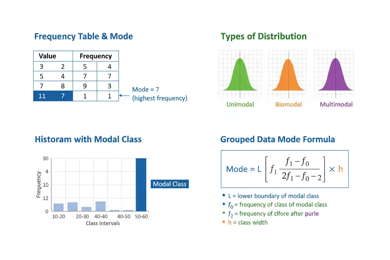
The mode is a measure of central tendency that identifies the value, category, or region occurring most frequently in a data set or having the greatest probability concentration in a probability distribution. Unlike the arithmetic mean, which combines every numerical magnitude, or the median, which depends on ordered position, the mode is determined by frequency: whichever value occurs most often is the mode, provided one value has a uniquely highest frequency. This makes the mode especially useful for categorical data, discrete numerical observations, repeated measurements, product choices, survey responses, and other situations in which the most common outcome matters more than a numerical balance point. A data set can have one mode, several modes, or no unique mode, while a continuous distribution defines its mode through the location where its probability density reaches a maximum rather than through repeated exact observations. Because frequency patterns can change substantially with sample size, grouping rules, rounding, or bin width, the mode is simple to understand but requires careful interpretation when data are continuous or when several frequencies are close.
The mode is one of the foundational measures of center within descriptive statistics and the broader Statistics & Probability framework. Its main strength is that it answers a question other averages do not: what outcome occurs most often? That question can be meaningful even when arithmetic averaging is impossible, which is why the mode works naturally with nominal categories as well as numerical values.
What Is the Mode?
The mode is the observation or category with the greatest frequency.
Suppose the data are:
2, 3, 3, 4, 5
The value:
3
appears twice, while every other value appears once.
Therefore:
Mode = 3
The calculation does not involve addition, division, or averaging.
It requires only a comparison of frequencies.
Basic Mode Rule
If a value xᵢ occurs with frequency fᵢ, the mode is the value whose frequency is largest.
Conceptually:
Mode = value associated with max(fᵢ)
For a discrete probability distribution, the population mode can similarly be defined as the value x maximizing the probability mass function:
Mode = arg maxₓ P(X = x)
For a continuous distribution with probability density function f(x), a mode is a point at which:
f(x)
reaches a maximum.
These definitions express the same central idea: the mode identifies greatest concentration.
Simple Mode Example
Consider:
5, 7, 8, 8, 8, 10, 12
Frequencies are:
5 → 1
7 → 1
8 → 3
10 → 1
12 → 1
The largest frequency is:
3
and it belongs to:
Therefore:
Mode = 8.
Mode From a Frequency Table
A frequency table makes mode identification especially easy.
Suppose:
| Value | Frequency |
|---|---|
| 1 | 4 |
| 2 | 7 |
| 3 | 12 |
| 4 | 9 |
| 5 | 3 |
The largest frequency is:
It belongs to:
Value = 3.
Therefore:
Mode = 3.
No other calculations are required.
Mode for Categorical Data
One major advantage of the mode is that it can summarize nominal categorical data.
Suppose customer selections are:
Basic, Premium, Basic, Standard, Premium, Premium, Basic, Premium
Count each category:
Basic = 3
Standard = 1
Premium = 4
Therefore:
Mode = Premium.
Calculating an arithmetic mean would make no sense because the category names have no meaningful numerical magnitudes.
The mode remains completely valid.
Why Mode Works for Nominal Variables
Nominal categories need only be distinguishable, not numerically ordered.
Examples include:
- colors;
- brands;
- countries;
- payment methods;
- product categories;
- operating systems.
If:
Blue
occurs more often than every other color, then:
Blue
is the mode.
No claim is being made that Blue is numerically greater or smaller than another category.
Frequency alone determines the result.
Mode for Ordinal Data
The mode also works for ordinal categories.
Suppose ratings are:
Poor, Fair, Good, Good, Good, Excellent
Then:
Mode = Good.
Because ordinal categories also have an order, the median may additionally be meaningful.
However, the two summaries answer different questions.
The mode identifies the most frequently chosen category, whereas the median identifies the central ranked category.
Mode for Discrete Numerical Data
Discrete numerical variables often have natural repeated values.
Suppose the number of customer orders per day is:
1, 2, 2, 2, 3, 3, 4, 5
The most frequently observed count is:
Therefore:
Mode = 2 orders.
This can be operationally useful because it describes the single most commonly observed workload rather than the arithmetic average workload.
Unimodal Data
A data set with exactly one most frequent value is called unimodal.
For example:
1, 2, 2, 2, 3, 4, 5
has:
Mode = 2.
No other value occurs three times.
Therefore, the sample is:
unimodal.
Many familiar theoretical distributions, including the ordinary normal distribution, are also unimodal because they possess one location of maximum density.
Bimodal Data
A data set is bimodal when two distinct values share the highest frequency.
Consider:
1, 2, 2, 3, 4, 4, 5
Frequencies are:
1 → 1
2 → 2
3 → 1
4 → 2
5 → 1
The greatest frequency is:
2
and both:
2 and 4
have that frequency.
Therefore:
Modes = 2 and 4.
The distribution is bimodal.
Why Bimodality Matters
Two modes can indicate more than an arithmetic curiosity.
They may suggest that the data combine two underlying groups or processes.
For example, commuting times could show one concentration among employees living near an office and another among employees traveling from distant suburbs.
A single arithmetic mean might fall between the two concentrations and describe relatively few actual observations.
The two modes reveal that the distribution has more than one preferred region.
Multimodal Data
A distribution with more than two distinct modes is called multimodal.
Consider:
1, 1, 2, 3, 3, 4, 5, 5
The highest frequency is:
Values:
1, 3, 5
all occur twice.
Therefore:
Modes = 1, 3, 5.
The sample is multimodal.
Multimodality often deserves investigation because it can reflect several populations, regimes, or recurring patterns.
No Unique Mode
A data set has no unique mode when no observation occurs more frequently than the others.
Consider:
1, 2, 3, 4, 5
Each value appears:
once.
Therefore, there is:
no unique mode.
Some descriptions simply say the data have “no mode.”
More precisely, every observation is tied at the same frequency, so no value stands out as more frequent.
Equal Frequencies Do Not Create a Useful Mode
Suppose:
2, 2, 4, 4, 6, 6.
All three distinct values have frequency:
Technically, each ties for the highest frequency.
However, calling all three values modes often conveys little useful information.
A clearer description is:
no unique modal value.
The purpose of reporting a mode is usually to identify meaningful frequency concentration.
When every category ties, that purpose is lost.
Mode vs Median
The median identifies the central ordered position, whereas the mode identifies the most frequent observation.
Consider:
1, 1, 2, 3, 4, 5, 6.
The mode is:
1
because it appears twice.
The median is:
3
because it is the fourth ordered observation.
Neither answer is wrong.
They describe different aspects of the same distribution.
Mode vs Arithmetic Mean
Consider:
1, 1, 1, 5, 10
Mode:
1
Arithmetic mean:
(1 + 1 + 1 + 5 + 10)/5
= 18/5
= 3.6.
The mode tells us which value occurs most often.
The mean tells us the numerical balance point.
The mean can be a value that does not occur at all.
The mode, for discrete raw data, must correspond to an observed value.
Mean, Median, and Mode Can Be Equal
Consider:
1, 2, 3, 3, 3, 4, 5.
Mode:
Median:
Mean:
(1 + 2 + 3 + 3 + 3 + 4 + 5)/7
= 21/7
= 3.
Therefore:
Mean = Median = Mode = 3.
This equality often occurs in highly symmetric unimodal data, but equality of the three statistics does not by itself prove that a distribution is normal.
Mean, Median, and Mode Can All Differ
Consider:
1, 2, 2, 3, 10.
Mode:
Median:
Mean:
18/5
= 3.6.
Now consider:
1, 1, 2, 4, 10.
Mode:
Median:
Mean:
18/5
= 3.6.
Thus:
Mode = 1
Median = 2
Mean = 3.6.
Each statistic captures a different feature of the distribution.
Mode and Skewness
For some smooth unimodal distributions, the relative positions of mean, median, and mode can provide a rough indication of skewness.
A commonly observed right-skew pattern is:
Mode < Median < Mean.
A common left-skew pattern is:
Mean < Median < Mode.
These relationships are not universal laws.
A distribution can violate them, particularly if it is multimodal, discrete, irregular, or highly unusual.
Distribution shape should be examined directly rather than inferred mechanically from three central statistics.
Mode and Histograms
For grouped continuous data, a histogram can reveal the region with the greatest concentration.
The class associated with the highest relevant bar is called the:
modal class.
When all class widths are equal, this is generally the class with the largest frequency.
If class widths differ, raw frequency alone can be misleading because wider intervals cover more numerical space.
In that case, frequency density should guide the graphical comparison.
The mode itself is owned here as a frequency concept; histogram construction is a separate graphical topic.
Modal Class
Suppose grouped frequencies are:
| Class | Frequency |
|---|---|
| 0–10 | 5 |
| 10–20 | 12 |
| 20–30 | 18 |
| 30–40 | 9 |
| 40–50 | 4 |
The greatest frequency is:
Therefore:
Modal class = 20–30.
This identifies an interval, not an exact numerical mode.
If the original observations are unavailable, further estimation is needed to locate a mode within the class.
Grouped-Data Mode Formula
For equal-width or suitably interpreted grouped continuous data with one clear modal class, a commonly used interpolation formula is:
Mode ≈ L + [(f₁ − f₀)/(2f₁ − f₀ − f₂)]h
where:
- L = lower class boundary of the modal class
- f₁ = frequency of the modal class
- f₀ = frequency of the class immediately before it
- f₂ = frequency of the class immediately after it
- h = width of the modal class
An equivalent form uses:
d₁ = f₁ − f₀
d₂ = f₁ − f₂
and:
Mode ≈ L + [d₁/(d₁ + d₂)]h.
The result is an interpolation estimate rather than an exact recovered raw-data value.
Grouped Mode Example
Suppose:
| Class | Frequency |
|---|---|
| 0–10 | 4 |
| 10–20 | 9 |
| 20–30 | 15 |
| 30–40 | 11 |
| 40–50 | 5 |
The modal class is:
20–30.
Use:
L = 20
f₁ = 15
f₀ = 9
f₂ = 11
h = 10.
Then:
Mode ≈ 20 + (15 − 9)/(2(15) − 9 − 11)
Simplify:
Mode ≈ 20 + 6/(30 − 20)
= 20 + (6/10)(10)
= 20 + 6
= 26.
Therefore:
Grouped mode ≈ 26.
Equivalent d₁ and d₂ Calculation
Using the same example:
d₁ = 15 − 9
= 6
and:
d₂ = 15 − 11
= 4.
Then:
Mode ≈ 20 + 6/(6 + 4)
= 20 + 6
= 26.
Both forms produce the same estimate.
The d₁/d₂ form makes the interpolation intuition particularly clear because it compares how much the modal frequency exceeds the frequencies on either side.
Why Grouped Mode Is an Estimate
Suppose the 20–30 class contains:
15 observations.
The frequency table does not reveal their precise values.
They could cluster around:
21,
around:
29,
or around some internal point.
The interpolation formula estimates the local peak using neighboring class frequencies.
It cannot reconstruct exact observations that were lost during grouping.
Therefore, reporting:
Mode ≈ 26
is more appropriate than implying:
Mode = 26 exactly.
Unequal Class Widths
If histogram classes have unequal widths, the largest raw frequency does not necessarily identify the greatest concentration.
Suppose:
| Class | Width | Frequency |
|---|---|---|
| 0–10 | 10 | 10 |
| 10–30 | 20 | 16 |
| 30–40 | 10 | 12 |
Raw frequency is largest in:
10–30.
But frequency densities are:
10/10 = 1
16/20 = 0.8
12/10 = 1.2.
The greatest density occurs in:
30–40.
Therefore, unequal-width grouped data require additional care before identifying a modal region.
Continuous Data Often Have No Repeated Exact Values
Suppose precise measurements are:
2.143
2.198
2.214
2.267
2.311.
Every observation may occur only once.
Calling the sample “without a mode” can be technically correct under an exact-value frequency definition, but it may miss the underlying distributional concentration.
For continuous data, modes are often estimated through:
- histogram peaks;
- density estimation;
- fitted probability models.
This is fundamentally different from simply counting repeated exact values in discrete data.
Mode of a Continuous Probability Distribution
For a continuous random variable with density f(x), a mode is a value xₘ satisfying:
f(xₘ) ≥ f(x)
for all relevant x, at least for a global mode.
The density value:
f(xₘ)
is not itself a probability at that exact point.
For a continuous distribution:
P(X = xₘ) = 0
under ordinary continuous probability models.
The mode therefore identifies the location of maximum density, not a point with positive probability mass.
Normal Distribution Mode
For a normal distribution:
X ~ N(μ, σ²),
the density is symmetric and reaches its unique maximum at:
x = μ.
Therefore:
Mode = μ.
The population mean and median are also:
μ.
Thus, for the normal distribution:
Mean = Median = Mode = μ.
This is a theoretical population property, not a guarantee that the sample mean, sample median, and empirical mode will be identical in finite data.
Uniform Distribution and Mode
A continuous uniform distribution has constant density across its support.
For:
X ~ Uniform(a, b),
every point between a and b has the same density.
Therefore, there is no unique mode.
Depending on terminology, every point in the interval can be considered modal because every point attains the maximum density.
This illustrates why “mode” does not always mean one preferred numerical location.
Mode of a Discrete Probability Distribution
For a discrete random variable, the mode is the outcome with the largest probability.
Suppose:
| x | P(X=x) |
|---|---|
| 0 | 0.10 |
| 1 | 0.25 |
| 2 | 0.40 |
| 3 | 0.25 |
The largest probability is:
0.40
at:
x = 2.
Therefore:
Mode = 2.
If two outcomes both had probability 0.40 and no outcome exceeded them, the distribution would have two modes.
Binomial Distribution Mode
For:
X ~ Binomial(n, p),
a mode can be described using:
(n + 1)p.
If:
(n + 1)p
is not an integer, the unique mode is:
floor[(n + 1)p].
If:
(n + 1)p
is an integer k, there are generally two adjacent modes:
k − 1
and:
k,
subject to ordinary parameter conditions.
This is an example where a probability model yields the mode analytically rather than through observed frequency counting.
Poisson Distribution Mode
For:
X ~ Poisson(λ),
if λ is not an integer:
Mode = floor(λ).
If λ is a positive integer:
Modes = λ − 1 and λ.
For example, if:
λ = 4.7,
then:
Mode = 4.
If:
λ = 5,
then:
Modes = 4 and 5.
The theoretical distribution can therefore be bimodal at adjacent integer values under specific parameter values.
Categorical Mode Does Not Need Numbers
Suppose a survey asks for preferred payment method:
Card, Cash, Card, Mobile, Card, Cash.
Frequencies are:
Card = 3
Cash = 2
Mobile = 1.
Therefore:
Mode = Card.
There is no need to encode:
Card = 1
Cash = 2
Mobile = 3.
Doing so would add arbitrary numerical meaning that the categories do not possess.
Frequency alone is sufficient.
Mode and Missing Categories
A category with zero observed frequency cannot be the sample mode.
Suppose predefined categories are:
A, B, C, D
but observations occur only in:
A, B, C.
If:
D = 0 observations,
then D contributes no empirical frequency concentration.
However, its absence can still be substantively important if the category was expected to appear.
A mode summarizes what occurred most often, not whether every theoretically possible outcome appeared.
Mode With Missing Data
Missing observations should generally be treated explicitly rather than silently turned into a category or numerical zero.
Suppose:
Yes = 40
No = 30
Missing = 50.
If “Missing” represents unavailable information rather than a substantive response category, describing:
Missing
as the mode would answer a data-quality question rather than the intended response question.
The appropriate denominator and treatment depend on the analysis.
Missingness should not be confused with an observed category unless it is intentionally being analyzed as one.
Mode and Sample Size
A sample mode can be unstable when n is small.
Suppose:
2, 2, 3, 4, 5
has mode:
Adding just two observations:
3, 3
changes the frequencies to:
2 → 2
3 → 3
so the mode becomes:
The sample mode can therefore shift abruptly even when only a small number of new observations are added.
This instability is one limitation of frequency-based central tendency.
Frequency Differences Matter
Consider:
A = 101 observations
B = 100 observations.
The mode is:
A.
But the difference is only:
one observation.
Calling A overwhelmingly dominant would exaggerate the evidence.
A mode reports which outcome is most frequent, not how strongly it dominates.
Frequency counts or percentages should accompany the mode when the difference between leading categories matters.
Strong vs Weak Modal Concentration
Compare two samples.
Sample A:
Category X = 90%
Category Y = 10%.
Sample B:
Category X = 51%
Category Y = 49%.
Both have:
Mode = X.
However, their concentration is very different.
In Sample A, X is overwhelmingly dominant.
In Sample B, the two categories are nearly tied.
Therefore, a reported mode is often more informative when paired with its frequency or relative frequency.
Relative Frequency of the Mode
If modal frequency is:
f_mode
and total sample size is:
n,
the modal proportion is:
p_mode = f_mode/n.
For example:
f_mode = 45
n = 100.
Then:
p_mode = 45/100
= 0.45
or:
45%.
This does not change which value is the mode, but it indicates how much of the sample actually occupies that modal value.
Can the Mode Be an Extreme Value?
Yes.
Consider:
100, 100, 100, 1, 2, 3, 4.
The mode is:
100
because it appears three times.
It also happens to be the maximum.
There is no rule requiring the mode to lie near the middle of the numerical range.
“Measure of central tendency” means it summarizes concentration, not that the mode must geometrically occupy the center.
Can the Mode Be the Minimum?
Yes.
Consider:
1, 1, 1, 4, 7, 10.
The mode is:
It is also:
Minimum = 1.
The median is:
(1 + 4)/2
= 2.5.
The arithmetic mean is:
24/6
= 4.
This example shows that different measures of center can occupy very different parts of an asymmetric distribution.
Can the Mode Be the Maximum?
Yes.
For:
1, 2, 5, 9, 9, 9
we have:
Mode = 9
and:
Maximum = 9.
The mode simply identifies the greatest frequency.
Its numerical rank is irrelevant to the definition.
Mode and Outliers
The mode is often resistant to isolated extreme numerical values because an observation occurring once usually does not change which value has the highest frequency.
Suppose:
2, 2, 2, 3, 4
has:
Mode = 2.
Replace 4 with:
1,000,000.
The mode remains:
However, repeated extreme values can themselves become the mode, so the statistic is not universally immune to unusual observations.
Mode and Outlier Detection
Formal outlier detection should not be based solely on whether an observation differs from the mode.
Suppose a continuous sample has no repeated values.
Every observation differs from every other one, yet that does not make every value an outlier.
Likewise, a value far from the modal region can be a legitimate member of a long-tailed distribution.
Outlier assessment requires an appropriate measure of distance, distributional context, robust method, or domain-specific rule.
Mode indicates concentration, not anomaly status.
Mode and Median Absolute Deviation
Median absolute deviation measures robust numerical spread around the median, whereas the mode identifies the most frequently occurring value.
A data set can have:
Mode = 5
while:
MAD = 20.
That would indicate the most common value is 5 but the central distribution is widely dispersed.
Conversely, a data set can have no unique mode while possessing a very small MAD.
The statistics are independent descriptive features.
Mode and Population Variance
Population variance measures the average squared deviation from the population mean, whereas the mode is determined entirely by maximum frequency or density.
Two populations can have the same mode and radically different variances.
For example, both might peak at:
10
while one is tightly concentrated between 9 and 11 and another extends from −100 to 200.
The shared modal location tells us nothing by itself about their overall dispersion.
Mode and Margin of Error
A margin of error describes sampling uncertainty around an estimated parameter under a specified inferential procedure, whereas the sample mode is primarily a descriptive frequency statistic.
There is no universal formula such as:
Mode ± 1.96(SE)
that applies automatically.
Inference for a population mode can be technically challenging, especially for continuous distributions where the estimated modal location may depend on density estimation or smoothing.
A sample’s most common value should therefore not be presented with a conventional mean-style margin unless a valid mode-specific method has been defined.
Mode Is Not a Measure of Spread
Suppose:
Data A = 4, 4, 4, 5, 5
and:
Data B = 4, 4, 4, 100, 1000.
Both have:
Mode = 4.
Yet their numerical spread differs enormously.
The mode does not encode:
- variance;
- standard deviation;
- range;
- IQR;
- MAD.
It describes concentration at the most frequent outcome only.
Additional statistics are required for dispersion.
Mode Is Not a Measure of Sample Size
Suppose two samples have:
Mode = 20.
One sample might contain:
10 observations
and another:
10 million.
The mode alone contains no information about n.
Likewise, it does not reveal whether the modal value appears:
2 times
or:
2 million times.
Report frequency or proportion when modal strength matters.
Mode Is Not Necessarily Unique
Unlike an ordinary arithmetic mean, which is unique whenever finite numerical values are averaged in the usual way, a mode can occur at several values.
This is not a flaw.
Multiple modes reveal genuine frequency structure.
If:
10
and:
50
are both strong peaks, forcing one numerical average between them could be less informative than reporting both modal regions.
Multimodality is itself useful information.
Mode and Data Grouping
Grouping can create or destroy apparent modes.
Suppose raw continuous data have two close clusters.
Using very wide intervals can merge them into one modal class.
Using narrower intervals can reveal two distinct peaks.
Conversely, extremely narrow intervals in a small sample can create random local peaks that look like separate modes.
The apparent grouped mode therefore depends partly on how the data are partitioned.
Mode and Rounding
Measurement rounding can create repeated values that would not occur at higher precision.
Suppose actual measurements are:
10.21, 10.24, 10.29, 10.31.
Rounded to one decimal place, they become:
10.2, 10.2, 10.3, 10.3.
The rounded data are bimodal:
10.2 and 10.3.
At full precision, there was no repeated exact value.
Thus, sample mode can partly reflect measurement resolution.
Heaping
Heaping occurs when observations cluster artificially at convenient rounded values.
For example, self-reported weights may disproportionately end in:
0
or:
Those rounded values can become modes even when the underlying continuous measurements have a smoother distribution.
A modal spike should therefore be interpreted in light of how values were measured and recorded.
The mode can reveal reporting behavior as well as underlying population structure.
Mode of Continuous Data and Histogram Bins
A histogram’s tallest equal-width bar identifies the most populated interval.
However, its midpoint is not automatically the exact mode.
Suppose the modal interval is:
20–30.
Reporting:
Mode = 25
solely because 25 is the midpoint assumes a structure not contained in the data.
A grouped interpolation formula or density estimate can provide a more reasoned estimate, but exact raw-data information has already been lost.
Kernel Density Mode
For continuous data, a smoothed density estimate can be used to identify a modal location.
Conceptually, the estimated mode is:
x̂_mode = arg maxₓ f̂(x)
where:
f̂(x)
is an estimated density.
The result can depend materially on the smoothing bandwidth.
Too much smoothing can merge separate peaks.
Too little smoothing can create many artificial local peaks.
Thus, continuous mode estimation requires methodological choices beyond simple frequency counting.
Global Mode vs Local Modes
A multimodal density can have several local maxima.
The global mode is the location with the highest density overall.
A local mode is a peak higher than nearby density values but not necessarily the highest peak in the entire distribution.
For example, a mixture distribution could have peaks at:
20
and:
80,
with the peak at 20 slightly higher.
Then 20 is the global mode, while both 20 and 80 are local modal locations.
The distinction matters in complex distributions.
Population Mode vs Sample Mode
A population can have one theoretical mode while a finite sample appears to have another.
Suppose the population’s most probable discrete value is:
Random sampling can nevertheless produce a sample in which:
4
occurs most frequently.
As n increases, sample frequencies may better approximate population probabilities under suitable random sampling, but no finite sample guarantees the population mode.
A sample mode is therefore an estimator or descriptive statistic, not an infallible population fact.
Instability When Probabilities Are Close
Suppose a population has:
P(X = A) = 0.34
P(X = B) = 0.33
P(X = C) = 0.33.
The population mode is:
A.
However, sample frequencies can easily place B or C first in a modest sample because their probabilities are nearly identical.
Mode estimation becomes difficult when the largest underlying probabilities differ only slightly.
A frequency winner does not necessarily imply a strong population preference.
Mode and Survey Responses
Suppose survey responses are:
| Response | Count |
|---|---|
| Strongly disagree | 12 |
| Disagree | 18 |
| Neutral | 25 |
| Agree | 41 |
| Strongly agree | 24 |
The modal category is:
Agree
because:
41
is the largest count.
The modal proportion is:
41/120
≈ 34.17%.
Therefore, “Agree” is the most common response even though it does not represent a majority of respondents.
Mode and majority are different concepts.
Mode vs Majority
A majority requires more than:
50%
of observations.
A mode requires only the largest frequency.
Suppose election preferences are:
Candidate A = 40%
Candidate B = 35%
Candidate C = 25%.
Candidate A is the modal choice.
But:
40% < 50%,
so Candidate A does not have a majority.
This distinction is important whenever several categories divide the total.
Mode and Plurality
In categorical decision contexts, the mode often corresponds to the plurality outcome: the category receiving more observations than any competitor, even if it receives less than half the total.
Thus:
modal category
and:
plurality category
can coincide.
However, “mode” is a statistical description, while “plurality” is often used in voting or decision rules.
The concepts arise from the same maximum-frequency structure but belong to different contexts.
Can the Mode Be a Decimal?
Yes.
Consider:
1.2, 1.4, 1.4, 1.4, 2.0.
The mode is:
1.4.
Any observed numerical value can be modal if it occurs most frequently.
For grouped continuous data, an estimated modal value can also be decimal even when class boundaries are whole numbers.
Can the Mode Be Negative?
Yes.
Consider:
−5, −5, −5, −2, 0, 3.
The mode is:
−5.
Frequency does not depend on sign.
Negative, zero, and positive values are treated identically for mode calculation.
Can Zero Be the Mode?
Yes.
Suppose:
0, 0, 0, 1, 2, 5.
Then:
Mode = 0.
Zero has no special restriction.
If it is the most frequently observed value, it is the mode.
This can be common in zero-inflated count data where many observations contain no events.
Zero-Inflated Data
A count variable may have an unusually large number of zeros.
Suppose:
60%
of observations are zero while the remaining values range from 1 to 20.
Then:
Mode = 0.
This tells us that “no event” is the most common individual outcome.
However, it does not describe the shape of the positive observations.
A zero-inflated model or separate analysis of nonzero values may provide additional insight.
Mode and Open-Ended Classes
Suppose grouped categories include:
Under 20
20–40
40–60
60+.
The modal class can still be identified by frequency if class widths and interpretations are comparable.
However, interpolating an exact grouped mode inside an open-ended modal class is problematic because its boundary or width may be unknown.
The class itself can still be reported as modal.
An exact numerical estimate requires additional information.
Mode and Ties
Tie handling should be transparent.
If two categories each occur:
25 times
and no other category exceeds:
25,
report both as modes rather than arbitrarily selecting one.
If many categories tie for the maximum, stating:
“No unique mode”
is often clearer.
An arbitrary tie-breaking rule converts a descriptive statistic into something different.
Mode in a Two-Value Data Set
Suppose:
2, 5.
Each value occurs once.
Therefore, neither occurs more frequently than the other.
There is no unique mode.
The median, by contrast, is:
(2 + 5)/2
= 3.5.
This simple example shows why the mode cannot always provide a single measure of center.
Mode With One Observation
For:
7
the only observed value also has the largest observed frequency:
Therefore, it can be described as the sample mode.
It is also:
mean = 7
median = 7
minimum = 7
maximum = 7.
The calculation is trivial, but a one-observation sample provides essentially no stable information about the distribution of a larger population.
Mode and Linear Transformations
Suppose a numerical sample has a unique mode:
M.
Apply a one-to-one linear transformation:
Y = aX + b
with:
a ≠ 0.
Every occurrence of M transforms into:
aM + b,
and frequency counts remain unchanged.
Therefore:
Mode(Y) = aM + b
for the transformed discrete sample.
The modal frequency is unchanged because one-to-one transformation preserves multiplicities.
Transformation Example
Suppose temperatures in degrees Celsius have sample mode:
20°C.
Convert to Fahrenheit:
F = 1.8C + 32.
Then:
Mode(F) = 1.8(20) + 32
= 68°F.
Every original observation equal to 20°C becomes 68°F, so its frequency is preserved.
This straightforward property applies to one-to-one transformations of raw discrete values.
Non-One-to-One Transformations Can Change the Mode
Suppose:
X = −2, −1, 1, 2
with each value occurring once.
There is no unique mode.
Apply:
Y = X².
Then:
Y = 4, 1, 1, 4.
Now:
Modes = 1 and 4.
The squaring transformation combines positive and negative values into the same outcomes, changing frequencies.
Thus, transformations that merge different input values can alter modal structure substantially.
Mode and Sample Frequency Distribution
The most direct calculation method is often to build a frequency table.
For observations xᵢ:
- identify distinct values;
- count occurrences;
- compare frequencies;
- select every value tied for the greatest frequency.
If:
max frequency
occurs once, the sample is unimodal.
If it occurs at two distinct values, the sample is bimodal.
If several values tie, the distribution is multimodal or has no informative unique mode.
Full Raw-Data Worked Example
Consider:
4, 7, 7, 8, 9, 9, 9, 10, 10, 12, 15
Step 1: Count Frequencies
4 → 1
7 → 2
8 → 1
9 → 3
10 → 2
12 → 1
15 → 1
Step 2: Identify the Maximum Frequency
max(f) = 3.
Step 3: Identify Its Value
The frequency:
3
belongs to:
Therefore:
Mode = 9.
The sample is unimodal.
Full Bimodal Example
Consider:
1, 2, 2, 3, 3, 4, 5
Frequencies are:
1 → 1
2 → 2
3 → 2
4 → 1
5 → 1.
The maximum frequency is:
Both:
2 and 3
share that maximum.
Therefore:
Modes = 2 and 3.
There is no defensible reason to choose one over the other without introducing a new criterion unrelated to the definition of mode.
Full Categorical Example
Suppose a store records preferred delivery options:
| Delivery Option | Customers |
|---|---|
| Standard | 120 |
| Express | 85 |
| Pickup | 140 |
| Same Day | 55 |
The greatest count is:
140
for:
Pickup.
Therefore:
Modal delivery option = Pickup.
Total customers:
120 + 85 + 140 + 55
= 400.
Modal proportion:
140/400
= 0.35
or:
35%.
Pickup is the most common option but does not represent a majority.
Full Grouped Mode Example
Suppose:
| Interval | Frequency |
|---|---|
| 0–10 | 5 |
| 10–20 | 12 |
| 20–30 | 20 |
| 30–40 | 14 |
| 40–50 | 7 |
The modal class is:
20–30.
Use:
L = 20
f₀ = 12
f₁ = 20
f₂ = 14
h = 10.
The grouped formula gives:
Mode ≈ L + [(f₁ − f₀)/(2f₁ − f₀ − f₂)]h
Substitute:
Mode ≈ 20 + (20 − 12)/(40 − 12 − 14)
= 20 + (8/14)(10)
= 20 + 5.714
≈ 25.71.
Therefore:
Estimated grouped mode ≈ 25.71.
Interpret the Grouped Estimate
The class:
20–30
contains the highest frequency.
The neighboring frequencies are:
12
and:
Because the upper neighboring class is somewhat more frequent than the lower neighboring class, the interpolation places the estimated mode above the exact midpoint:
The estimate:
25.71
is therefore consistent with a local peak leaning slightly toward the upper side of the modal interval.
It remains an approximation based on grouped data.
Common Mode Mistakes
A common mistake is confusing the mode with the largest numerical value. The mode is the value with the largest frequency, not the largest magnitude.
Another mistake is assuming every data set must have exactly one mode. Samples can be bimodal, multimodal, or lack a unique mode.
Analysts also sometimes average tied modes and call the result the mode. If values 2 and 8 are both modal, their average 5 is not automatically a mode and may not occur at all.
For grouped data, treating the midpoint of the modal class as the exact mode ignores the uncertainty created by grouping.
When class widths differ, choosing the class with the highest raw frequency can misidentify the region of greatest density.
Another error is using the mode alone to describe highly multimodal data when the multiple peaks themselves are the important finding.
Finally, continuous measurements should not be declared meaningfully “mode-free” simply because no two high-precision sample values happen to be identical; the underlying density can still have a clear modal region.
How to Calculate the Mode Step by Step
For raw categorical or discrete numerical data, list each distinct value or category and count its occurrences.
Identify:
max(frequency).
Then determine which value or values have that frequency.
If one value has the maximum:
one mode.
If two values share it:
bimodal.
If several share it:
multimodal or no unique mode.
For grouped continuous data, identify the modal class and use an appropriate density comparison when class widths differ. If a numerical estimate inside an equal-width modal class is required, a grouped interpolation formula can be used with its assumptions stated clearly.
When Mode Is Most Useful
Mode is especially useful when the analytical question asks for:
- the most common category;
- the most common discrete value;
- the most popular choice;
- the most frequent event count;
- the dominant size or product type;
- the peak of a probability distribution;
- modal regions in grouped data.
It is also the only traditional central-tendency measure that works directly with nominal categories.
When the practical question is “what occurs most often?”, the mode is usually the natural answer.
When Mode Is Less Useful
Mode can be less informative when:
- almost every continuous observation is unique;
- several frequencies are nearly tied;
- bin choices strongly affect a grouped modal class;
- the distribution is highly multimodal;
- a numerical balance point is required;
- total magnitude matters.
In these situations, other measures and visualizations can provide more stable information.
The mode should be chosen because frequency concentration matters, not merely because it is one of the standard measures of center.
How to Report the Mode
For a discrete sample, a clear report can state:
“The mode was 9, occurring three times.”
For categorical data:
“Pickup was the modal delivery option, selected by 140 of 400 customers, or 35%.”
For several modes:
“The sample was bimodal, with modes at 2 and 3.”
For grouped data:
“The modal class was 20–30, with an interpolated grouped mode of approximately 25.71.”
Reporting frequency or proportion alongside the mode often provides important context about how dominant the modal outcome actually is.
Frequently Asked Questions About Mode
What is the mode?
The mode is the value, category, or distribution location with the greatest frequency or probability concentration.
How do you calculate the mode?
Count how often each value occurs and identify the value with the highest frequency.
Is there a basic mode formula?
Conceptually:
Mode = value associated with max(frequency)
What is the mode of 1, 2, 2, 3?
2
Can there be two modes?
Yes. A distribution with two distinct highest-frequency values is bimodal.
Can there be more than two modes?
Yes. It is then multimodal.
Can a data set have no mode?
Yes, if no value has a uniquely greater frequency than the others.
Is the mode always one of the observations?
For discrete raw sample data, yes.
Can a grouped-data mode be a value not directly observed?
Yes. Interpolation can estimate a numerical location inside the modal class.
Can the mode be categorical?
Yes.
Can the mode be used for nominal data?
Yes. This is one of its greatest advantages.
Can the mean be used for nominal data?
No, not meaningfully when category codes have no quantitative interpretation.
Can the median be used for nominal data?
Generally no, because nominal categories have no natural order.
Can the mode be used for ordinal data?
Yes.
Can the mode be negative?
Yes.
Can zero be the mode?
Yes.
Can the mode be a decimal?
Yes.
Can the mode equal the minimum?
Yes.
Can the mode equal the maximum?
Yes.
Is the mode the largest value?
No. It is the most frequent value.
Is mode the same as median?
No. Median identifies central rank.
Is mode the same as mean?
No. Mean is the arithmetic balance point.
Can mean, median, and mode all be equal?
Yes.
Does equality of mean, median, and mode prove normality?
No.
What is a unimodal distribution?
A distribution with one mode.
What is a bimodal distribution?
A distribution with two modes or two major density peaks.
What is a multimodal distribution?
A distribution with several modes or peaks.
What can multimodality indicate?
It can suggest multiple subpopulations, regimes, or processes, although sampling noise and grouping should also be considered.
What is a modal class?
The grouped interval containing the greatest relevant frequency concentration.
What is the grouped-data mode formula?
A common interpolation formula is:
Mode ≈ L + [(f₁ − f₀)/(2f₁ − f₀ − f₂)]h
What do f₀, f₁, and f₂ mean?
f₁ = modal-class frequency
f₀ = preceding-class frequency
f₂ = following-class frequency.
Is grouped mode exact?
Usually not.
Why not?
Grouping hides the exact locations of observations inside each class.
Can unequal class widths affect the modal class?
Yes. Frequency density may need to be considered rather than raw frequency.
What is the mode of a continuous distribution?
It is a location where the probability density reaches a maximum.
Does a continuous variable need repeated exact observations to have a mode?
No.
What is the mode of a normal distribution?
μ
which is also its mean and median.
Does a uniform distribution have one unique mode?
A continuous uniform distribution does not have a unique mode because density is constant across its support.
Can a theoretical distribution have two modes?
Yes.
What is the mode of a Poisson distribution?
If λ is not an integer:
floor(λ).
If λ is a positive integer, the adjacent values:
λ − 1 and λ
are modes.
Is mode affected by outliers?
An isolated extreme observation often has little effect, but repeated extreme observations can become modal.
Is the mode robust?
It can be resistant to extreme magnitudes, but it may be unstable with respect to small changes in frequencies.
Why can sample mode be unstable?
A few new observations can change which value has the largest frequency.
Does mode measure variability?
No.
Does mode tell you sample size?
No.
Does mode tell you how dominant the most frequent value is?
Not by itself.
What should be reported with mode?
Its frequency or relative frequency is often useful.
Is the modal category always a majority?
No.
What is the difference between mode and majority?
A mode only needs to occur more frequently than each alternative. A majority requires more than 50% of observations.
Can the mode change when values are rounded?
Yes.
Why?
Rounding can combine distinct measurements into repeated displayed values.
Can histogram binning change an apparent mode?
Yes.
Can changing bin width create or hide multiple peaks?
Yes.
Is the midpoint of the modal class automatically the mode?
No.
Can mode be estimated with density methods?
Yes, continuous-data modes can be estimated from smoothed density functions.
What is a global mode?
The location attaining the highest density or probability overall.
What is a local mode?
A local peak that exceeds nearby values but may not be the highest peak globally.
Is the sample mode guaranteed to equal the population mode?
No.
What happens when population category probabilities are nearly tied?
Sample mode can change frequently across samples.
Can a mode have a confidence interval?
Inference for a population mode is possible, but there is no universal mean-style margin-of-error formula that applies automatically.
Does mode help identify outliers?
It can show where data concentrate, but observations far from the mode are not automatically outliers.
How does mode differ from median absolute deviation?
Mode identifies maximum frequency, while median absolute deviation measures robust numerical spread around the median.
How does mode differ from population variance?
Mode describes frequency concentration; variance describes average squared dispersion around the population mean.
What is the main advantage of the mode?
It identifies the most common outcome and works naturally with categorical data where arithmetic averages are meaningless.
What is its main limitation?
It can be non-unique or unstable, and for continuous data its apparent location can depend strongly on measurement precision, grouping, or smoothing choices.
What is the most important rule when calculating the mode?
Identify the outcome with the greatest frequency, report all meaningful ties rather than forcing a single answer, and distinguish an exact discrete mode from an estimated modal location obtained from grouped or continuous data.