
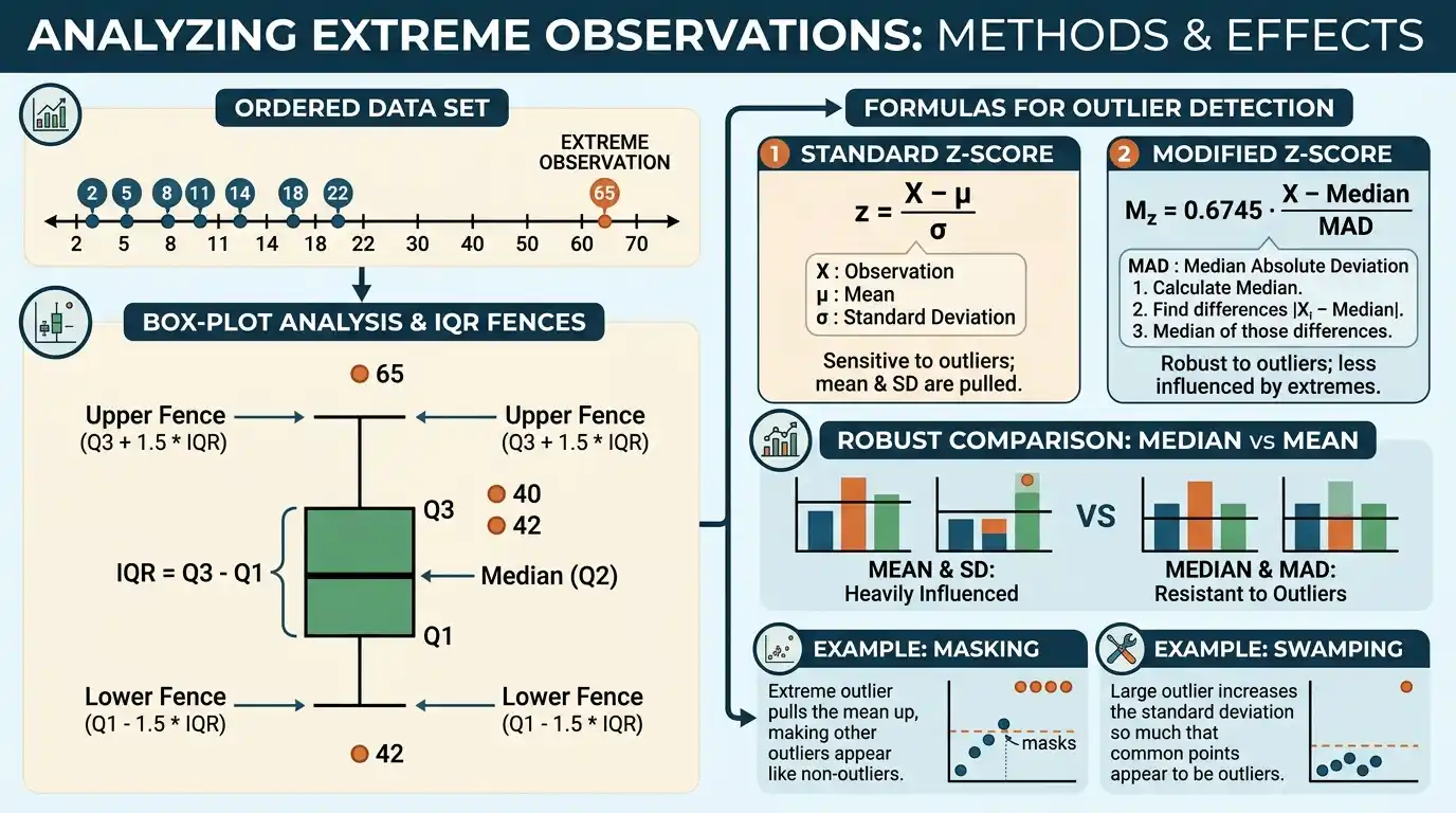

Outlier detection is the process of identifying observations that are unusually distant from the central pattern of a data set according to a defined statistical, mathematical, or domain-specific criterion. An outlier may be a genuine rare observation, a measurement or recording error, a member of a different population, evidence of a changed process, or simply an expected extreme value from a distribution with long tails, so detecting an unusual point is not the same as proving that the point is invalid. Common methods include the 1.5×IQR rule, ordinary z-scores, modified z-scores based on the median and median absolute deviation, model residuals, distance-based techniques, and multivariate procedures designed to identify unusual combinations of variables. The appropriate method depends strongly on distribution shape, sample size, dimensionality, measurement scale, and the purpose of the analysis, because a rule that works well for approximately symmetric univariate data can perform poorly for highly skewed, multimodal, discrete, or correlated data. Effective outlier detection therefore combines numerical screening with graphical examination and contextual validation rather than applying one universal threshold mechanically.
Outlier detection belongs to the broader framework of descriptive statistics within Statistics & Probability. It is especially important because unusual observations can materially affect means, variances, correlations, regression coefficients, forecasts, and statistical tests, yet indiscriminate removal of extreme values can distort the very distribution the analysis is supposed to describe.
What Is an Outlier?
An outlier is an observation that differs substantially from the pattern formed by most other observations.
Consider:
8, 9, 10, 10, 11, 12, 50
The value:
50
is far from the cluster between:
8 and 12.
It is therefore a plausible outlier.
However, statistical distance alone does not tell us whether 50 is:
- an incorrect entry;
- an unusual but valid observation;
- evidence of a separate subgroup;
- a natural tail observation.
Outlier detection identifies unusualness.
Interpretation determines what that unusualness means.
What Is the Purpose of Outlier Detection?
Outlier detection can serve several different goals.
One analyst may be looking for:
data-entry mistakes.
Another may want to detect:
fraud,
equipment failures,
unusual customers,
rare events,
or:
observations that violate a model’s assumptions.
These objectives are not interchangeable.
A value that is undesirable noise in one application may be the most important observation in another.
For example, a rare equipment failure should not be deleted merely because it is statistically unusual if detecting failures is the purpose of the analysis.
Outlier Detection Formula
There is no single universal outlier detection formula.
Common univariate rules include:
Lower fence = Q₁ − 1.5(IQR)
Upper fence = Q₃ + 1.5(IQR)
where:
IQR = Q₃ − Q₁
and the ordinary z-score:
zᵢ = (xᵢ − x̄)/s
as well as the modified z-score:
Mᵢ = 0.6745(xᵢ − Median)/MAD
where MAD is the raw median absolute deviation.
Each rule uses a different definition of center and spread.
Consequently, the same observation can be flagged by one method and not by another.
IQR Method for Outlier Detection
The interquartile range method is one of the most widely used robust rules.
First calculate:
IQR = Q₃ − Q₁
Then calculate the fences:
Lower fence = Q₁ − 1.5(IQR)
Upper fence = Q₃ + 1.5(IQR)
An observation is commonly flagged as a potential outlier if:
x < Lower fence
or:
x > Upper fence.
The word potential matters because the rule identifies statistical unusualness, not data invalidity.
Simple IQR Example
Consider:
2, 4, 5, 7, 8, 9, 10, 12, 13, 15, 40
There are:
n = 11
observations.
The central value is:
Using the median-of-halves convention that excludes the overall central observation:
Lower half:
2, 4, 5, 7, 8
so:
Q₁ = 5.
Upper half:
10, 12, 13, 15, 40
so:
Q₃ = 13.
Therefore:
IQR = 13 − 5
= 8.
Calculate the IQR Fences
Lower fence:
5 − 1.5(8)
= 5 − 12
= −7
Upper fence:
13 + 1.5(8)
= 13 + 12
= 25
Therefore, potential outliers satisfy:
x < −7
or:
x > 25.
The value:
40
exceeds the upper fence.
Therefore:
40 is flagged as a potential upper outlier.
No lower observation falls below −7.
Why the IQR Rule Is Robust
The IQR uses:
Q₁
and:
Q₃,
which depend primarily on ordered positions rather than the magnitude of the most extreme observations.
Suppose the value:
40
in the previous sample changes to:
4,000,000.
Under the same quartile convention:
Q₁ = 5
Q₃ = 13
and:
IQR = 8
remain unchanged.
The upper fence therefore remains:
The extreme value becomes vastly larger, but it does not inflate the detection threshold.
That resistance is one major advantage of the IQR method.
Inner and Outer Fences
A more elaborate box-plot convention distinguishes ordinary and extreme potential outliers.
Inner fences use:
Q₁ − 1.5(IQR)
and:
Q₃ + 1.5(IQR).
Outer fences use:
Q₁ − 3(IQR)
and:
Q₃ + 3(IQR).
Values beyond the outer fences are sometimes described as extreme outliers.
These labels are heuristic classifications.
They do not establish that observations beyond 3×IQR are erroneous.
Outer-Fence Example
Using:
Q₁ = 5
Q₃ = 13
IQR = 8
the outer upper fence is:
13 + 3(8)
= 13 + 24
= 37.
The observation:
40
also exceeds:
Therefore, it lies beyond the outer upper fence under this convention.
That makes it statistically very distant relative to the central quartile spread, but the next step is still investigation rather than automatic deletion.
Quartile Conventions Matter
Finite-sample quartiles can be calculated using several accepted conventions.
Different methods can produce slightly different:
Q₁
and:
Q₃.
Because:
IQR = Q₃ − Q₁,
the outlier fences can also change.
This matters especially in small samples where one rank or interpolated value can materially shift the boundary.
When exact reproducibility matters, state the quartile convention used rather than assuming every calculator implements the same one.
Z-Score Method
A z-score measures how many standard deviations an observation lies from the sample mean:
zᵢ = (xᵢ − x̄)/s
where:
- xᵢ = observation
- x̄ = sample mean
- s = sample standard deviation
A common informal rule flags observations satisfying:
|z| > 3.
Other thresholds are possible.
The method is most interpretable when mean and standard deviation provide meaningful summaries of the distribution.
Z-Score Example
Return to:
2, 4, 5, 7, 8, 9, 10, 12, 13, 15, 40
The sample mean is approximately:
x̄ ≈ 11.364.
The sample standard deviation is approximately:
s ≈ 10.279.
For:
x = 40,
the z-score is:
z = (40 − 11.364)/10.279
≈ 28.636/10.279
≈ 2.786.
Using the common:
|z| > 3
rule, 40 would not be flagged.
Yet the IQR rule does flag it.
Why the Z-Score Missed the Extreme Value
The observation:
40
raises both the sample mean and the sample standard deviation.
Because the z-score uses those same nonrobust statistics in its denominator and center, the extreme point partly changes the reference system against which it is judged.
This phenomenon is one form of:
masking.
The outlier increases the estimated spread enough to make itself look less unusual.
Robust procedures are designed partly to reduce this problem.
Modified Z-Score
A robust alternative uses the median and raw median absolute deviation:
Mᵢ = 0.6745(xᵢ − Median)/MAD
A commonly used screening threshold is approximately:
|Mᵢ| > 3.5.
The factor:
0.6745
calibrates raw MAD to an ordinary z-score-like scale under a normal reference distribution.
Because both median and MAD resist isolated extreme observations, modified z-scores can detect anomalies that ordinary z-scores partially mask.
Modified Z-Score Example
For the same data:
2, 4, 5, 7, 8, 9, 10, 12, 13, 15, 40
the median is:
Absolute deviations are:
7, 5, 4, 2, 1, 0, 1, 3, 4, 6, 31.
Sorted:
0, 1, 1, 2, 3, 4, 4, 5, 6, 7, 31.
Therefore:
MAD = 4.
For x = 40:
M = 0.6745(40 − 9)/4
= 0.6745(31)/4
≈ 20.9095/4
≈ 5.227.
Because:
5.227 > 3.5,
the observation is strongly flagged.
Why Modified Z-Scores Are Robust
The median absolute deviation depends on the middle absolute distance from the median rather than the average squared distance from the mean.
One extreme observation can therefore become enormously large without necessarily changing the MAD at all.
In the previous example:
MAD = 4
remains controlled by central observations.
Consequently, the observation 40 cannot inflate the robust denominator enough to hide itself.
This is a major advantage when contamination is sparse.
Median as a Robust Center
The median determines central rank rather than arithmetic balance.
Suppose the largest observation changes from:
40
to:
4,000.
The arithmetic mean changes substantially.
The median may remain:
A robust outlier procedure therefore uses a center that is not dragged strongly toward the extreme point being evaluated.
This reduces self-masking and makes anomaly scores more stable under isolated contamination.
MAD Equal to Zero
Modified z-scores require:
MAD > 0.
Consider:
5, 5, 5, 5, 6, 20, 100.
Median:
Absolute deviations:
0, 0, 0, 0, 1, 15, 95.
Therefore:
MAD = 0.
The modified z-score formula would require division by zero and is undefined.
This can occur naturally in highly tied or discrete data.
Another method must then be selected.
Ordinary Z-Scores vs Modified Z-Scores
Ordinary z-score:
z = (x − x̄)/s
uses:
mean + standard deviation.
Modified z-score:
M = 0.6745(x − median)/MAD
uses:
median + robust spread.
Ordinary z-scores can be efficient and informative when the data follow a suitable symmetric light-tailed distribution without problematic contamination.
Modified z-scores are more resistant when extreme observations are precisely what the analyst is trying to detect.
Neither rule is universally superior.
Outliers and Population Variance
Population variance measures average squared deviation from the population mean.
Because deviations are squared, an extreme value can contribute disproportionately to the variance.
Suppose most observations lie close to:
10
while one lies at:
1,000.
That distant observation can dramatically increase the mean-centered squared dispersion.
This is one reason variance-based outlier rules can behave differently from quartile- or MAD-based methods.
The choice of spread measure changes what counts as statistically distant.
Outliers and Range
The range is:
Maximum − Minimum.
It is completely determined by the two most extreme observations.
Therefore, an outlier can increase the range dramatically.
For:
2, 4, 5, 7, 8, 9, 10, 12, 13, 15, 40
the range is:
40 − 2
= 38.
If 40 changes to 4,000:
Range = 4,000 − 2
= 3,998.
This sensitivity makes range useful for describing full span but poor as a robust detection scale.
Outliers and Mode
The mode identifies the most frequently occurring value or category.
An isolated extreme observation usually has no effect on the mode because it appears only once.
For example:
5, 5, 5, 6, 7, 1000
still has:
Mode = 5.
However, a cluster of unusual values can itself create another mode.
Multimodality may indicate that observations considered “outliers” under a one-population assumption actually belong to a legitimate second subgroup.
Outlier vs Rare Observation
An observation can be rare without being anomalous.
Suppose a correctly specified probability model assigns a small but nonzero probability to very large values.
Eventually, a sufficiently large sample may contain them.
If they are generated legitimately by the same process, labeling them as data errors simply because they are rare would be incorrect.
Outlier detection should therefore distinguish:
statistical rarity
from:
data invalidity.
The two concepts overlap only when the evidence supports that interpretation.
Outlier vs Data Error
A data error is an observation that is wrong because of collection, recording, processing, or measurement failure.
Examples include:
- entering 500 instead of 50;
- recording centimeters as meters;
- duplicating a record;
- instrument malfunction;
- impossible dates or values.
An outlier can be a data error, but it does not have to be.
Conversely, some data errors are not statistically extreme and therefore may escape purely numerical outlier detection.
Data validation rules remain important.
Domain-Specific Impossible Values
Some anomalies can be identified without statistical thresholds.
For example, if a variable is defined as:
probability,
then valid values satisfy:
0 ≤ p ≤ 1.
A recorded value:
p = 1.4
is invalid by definition.
Likewise, a percentage intended to lie between:
0% and 100%
may reveal a coding problem if a value falls outside that domain.
Logical constraints can be more decisive than statistical distance.
Contextual Outliers
An observation can be ordinary globally but unusual within its context.
Suppose electricity use of:
500 kWh
is normal for a large building but extreme for a small apartment.
A global threshold could miss the anomaly if all property types are pooled.
Contextual outlier detection evaluates observations relative to:
- subgroup;
- season;
- location;
- operating state;
- expected condition.
This is especially important when heterogeneous populations are combined.
Collective Outliers
A group of observations can be unusual even when no single member is extreme.
Suppose a sensor normally alternates randomly around:
A sequence of:
50, 51, 50, 51, 50
may look ordinary point by point.
However, a very long uninterrupted pattern or unusual temporal sequence can be anomalous collectively.
Time-series and sequence-based detection therefore often evaluates patterns rather than isolated values.
Global Outliers
A global or point outlier is unusual relative to the complete data set without requiring special contextual information.
For example:
1, 2, 3, 4, 5, 1000
contains an obvious globally distant point.
Methods such as IQR fences and robust z-scores commonly target this type of anomaly.
Global rules are easiest to apply but can be misleading when the underlying data consist of several legitimate populations.
Univariate Outlier Detection
Univariate methods analyze one variable at a time.
Examples include:
IQR fences
z-scores
modified z-scores
percentile rules.
These methods are simple and interpretable.
However, they can miss observations that are unusual only because of relationships among several variables.
A point can look normal on each variable separately while being abnormal in combination.
Multivariate Outliers
Suppose height and weight are considered separately.
A particular height may be ordinary.
A particular weight may also be ordinary.
Yet their combination could be extremely unusual relative to the relationship between height and weight.
Multivariate outlier detection examines joint structure.
Common ideas include:
- Mahalanobis distance;
- robust covariance methods;
- nearest-neighbor distances;
- density-based methods;
- isolation methods.
The appropriate method depends on dimension and data structure.
Mahalanobis Distance
For a multivariate observation vector x with mean vector μ and covariance matrix Σ, Mahalanobis distance is:
D² = (x − μ)ᵀΣ⁻¹(x − μ)
This measure accounts for:
- variable scales;
- correlations among variables.
A point lying along a high-variance correlation direction can receive a smaller distance than a point equally far away in a low-variance direction.
That makes Mahalanobis distance more appropriate than ordinary Euclidean distance for some correlated multivariate data.
Why Euclidean Distance Can Mislead
Suppose two variables use very different units:
income in thousands
and:
age in years.
A raw Euclidean distance can be dominated by the numerically larger scale.
Likewise, strongly correlated variables contain redundant direction information.
Standardization can address scale, but correlation can still matter.
Mahalanobis-type methods incorporate covariance structure directly.
However, ordinary covariance estimates themselves can be distorted by multivariate outliers, motivating robust alternatives.
Outliers and Regression
In regression, several kinds of unusual observations should be distinguished.
A point can have:
a large residual,
meaning its observed response differs strongly from the fitted response.
It can have:
high leverage,
meaning its predictor values are unusual.
It can also be:
influential,
meaning removing it changes the fitted model substantially.
These concepts overlap but are not identical.
An observation with a large residual need not have high leverage, and a high-leverage point need not be influential if it follows the regression pattern closely.
Residual-Based Detection
For observation i:
Residual = yᵢ − ŷᵢ.
Large residuals indicate poor model fit for specific observations.
Standardized or studentized residuals put residuals on a scale adjusted for estimated variability.
Rules such as:
|studentized residual| > 2
or:
3
are sometimes used for screening.
These are heuristics rather than automatic deletion criteria.
Model assumptions and multiple-comparison considerations matter.
Leverage
Regression leverage measures how unusual an observation’s predictor values are relative to the rest of the design.
A point far from the center of predictor space can have high leverage even if its response lies close to the fitted regression line.
High leverage means the observation has the potential to influence the fit.
It does not by itself prove the response is anomalous.
Leverage and residual size should be considered together.
Influence
Influential observations materially affect model estimates.
Common diagnostics include:
- Cook’s distance;
- DFBETAS;
- DFFITS.
An observation can be influential because it combines:
unusual predictor values
with:
substantial residual discrepancy.
Influence is a model-specific idea.
A point that strongly changes one regression model might be entirely ordinary under another correctly specified model.
Time-Series Outliers
Time-series observations require attention to temporal structure.
A value can be unusual relative to:
- recent history;
- seasonality;
- trend;
- expected volatility.
For example, sales of:
1,000 units
might be extreme in February but normal during a major holiday season.
Simple global IQR rules can misclassify seasonal peaks.
Time-series outlier detection often works with residuals after trend and seasonal components have been modeled.
Seasonal Outliers
Suppose daily electricity demand has predictable summer peaks.
A high observation in July may be perfectly normal.
The same value in mild-weather months could be anomalous.
A contextual model can compare each observation with its seasonal expectation.
This illustrates an important principle:
unusualness is relative to the appropriate reference distribution.
Pooling fundamentally different operating conditions can create false outliers.
Outliers in Skewed Data
The ordinary 1.5×IQR rule is robust but can flag many valid observations in a naturally long-tailed skewed distribution.
For example, financial transaction values or waiting times may have genuine long upper tails.
A large value may exceed an upper quartile fence without being erroneous.
Potential alternatives include:
- transformation;
- asymmetric robust rules;
- distribution-specific models;
- quantile methods.
The method should respect the expected shape rather than forcing symmetry where none exists.
Log Transformation
For positive right-skewed data, a logarithmic transformation:
y = ln(x)
can compress very large values and turn multiplicative differences into additive differences.
Outlier screening can then be performed on the transformed scale when that scale is substantively meaningful.
A value that appears extraordinarily distant on the raw scale may be ordinary in multiplicative terms.
Transformation changes the question being asked, so it should be justified by the measurement structure rather than used solely to suppress inconvenient extremes.
Outliers in Heavy-Tailed Distributions
A heavy-tailed population naturally generates extreme observations more frequently than a normal model predicts.
Using:
|z| > 3
with an implicit normal interpretation can therefore label valid observations too aggressively.
In such settings, robust or distribution-specific methods can be more appropriate.
The existence of extreme observations is sometimes part of the phenomenon itself.
Removing them can make the sample look artificially light-tailed.
Outliers in Small Samples
Outlier detection is especially uncertain when n is very small.
Consider:
5 observations.
One value far from the other four might be:
- a genuine error;
- a legitimate fifth observation from a skewed population;
- evidence of two subgroups.
There is little information available to distinguish these explanations statistically.
Threshold rules can still be calculated, but they should be interpreted cautiously.
Showing the raw observations is often more informative than relying only on a label.
Outliers in Large Samples
Large samples naturally provide more opportunities to observe extreme values.
Suppose a normally distributed variable is sampled:
100 times
versus:
10 million times.
The second sample is much more likely to contain observations several standard deviations from the mean.
A fixed threshold may therefore flag many observations even when the model is correct.
Statistical unusualness should be interpreted relative to sample size and expected tail frequency.
Multiple Testing Problem
Suppose a procedure flags any observation with:
|z| > 3.
Under a standard normal model, such observations are rare individually.
But if millions of observations are tested, some extreme values are expected by chance.
The probability that at least one observation exceeds a threshold increases with the number of opportunities.
Therefore, large-scale anomaly detection often needs to control:
- false positive rates;
- expected number of alerts;
- operational review capacity.
A threshold cannot be interpreted independently of how many observations are screened.
Masking
Masking occurs when outliers distort the center or spread estimate enough to hide themselves or other outliers.
Suppose several large values inflate:
x̄
and:
s.
Their ordinary z-scores can become moderate because the reference distribution has shifted and widened toward them.
This is exactly why robust center and spread estimators are valuable.
They reduce the ability of a small contaminated subset to define its own permissive detection threshold.
Swamping
Swamping occurs when ordinary observations are incorrectly flagged because outliers have distorted the reference estimates.
For example, a cluster of extreme upper values can shift the mean upward.
Some legitimate lower observations may then appear artificially distant from that shifted center.
Thus, nonrobust procedures can both:
miss true anomalies
and:
create false ones.
Robust methods aim to reduce both effects when contamination is limited.
Example of Masking
Using the sample:
2, 4, 5, 7, 8, 9, 10, 12, 13, 15, 40
we found:
z(40) ≈ 2.786.
A simple:
|z| > 3
threshold does not flag 40.
Yet:
IQR upper fence = 25
and:
modified z ≈ 5.227.
Both robust methods flag the observation.
This disagreement demonstrates how a nonrobust standard deviation can become inflated by the very point being tested.
Consensus Across Methods
If several conceptually different methods all flag an observation, evidence of unusualness becomes stronger.
For example, suppose a point:
- exceeds the 1.5×IQR fence;
- has modified |z| > 3.5;
- appears isolated graphically;
- violates an expected operational range.
That combination deserves serious investigation.
However, even unanimous statistical flags do not prove the value is erroneous.
Domain validation remains necessary.
Disagreement Across Methods
Different methods can legitimately disagree because they define unusualness differently.
The IQR method evaluates distance relative to the central half of the sample.
Z-scores evaluate distance relative to mean and standard deviation.
MAD-based scores use robust median-centered scale.
Model-based procedures compare observations with expected values conditional on predictors.
A disagreement is therefore useful information about the distribution, not necessarily evidence that one method is wrong.
Graphical Outlier Detection
Graphs are valuable because numerical thresholds compress information.
Useful displays can include:
- box plots;
- histograms;
- scatterplots;
- residual plots;
- time-series plots.
A box plot can show quartile-based extremes.
A scatterplot can reveal multivariate patterns.
A time-series plot can reveal abrupt changes.
Graphs do not replace quantitative rules, but they often explain why a point has been flagged.
Box Plot and Outliers
A modified box plot commonly uses the 1.5×IQR rule.
The box spans:
Q₁ to Q₃.
The median appears inside the box.
Whiskers usually extend to the most extreme observed values that remain within the inner fences.
Values beyond the whiskers are plotted individually as potential outliers.
Therefore, whisker endpoints are not necessarily the minimum and maximum.
Histogram and Outliers
A histogram can show sparse tail bins or separated observations, but its ability to display individual extremes depends on bin width.
A very wide bin can hide an outlier inside a broad interval.
A very narrow bin can make ordinary tail observations look isolated.
Thus, apparent outliers should be checked under sensible alternative binning choices.
A graph’s resolution is part of its statistical interpretation.
Scatterplot Outliers
In two dimensions, scatterplots can reveal observations that depart from the joint relationship between variables.
Suppose most points follow:
y ≈ 2x.
A point with an ordinary x value and ordinary y value may still lie far from that relationship.
Univariate screening of x and y separately could miss it.
The scatterplot reveals the conditional anomaly.
This is one reason multivariate analysis cannot be replaced by independent one-variable rules.
Data Validation Before Statistical Detection
Before applying statistical outlier rules, verify basic data quality.
Useful checks include:
- valid type;
- valid unit;
- plausible range;
- duplicate records;
- impossible codes;
- missing-value conventions.
If a variable represents age in years and contains:
850,
a domain rule may identify the problem immediately.
There is no need to rely solely on an IQR or z-score threshold.
Logical validation and statistical detection complement each other.
Unit Errors
Suppose most heights are recorded in:
centimeters
but one observation is entered in:
meters.
Values might look like:
165, 172, 180, 1.75, 168.
The value:
1.75
would appear as an extreme low outlier even though the underlying measurement may be perfectly reasonable.
The real problem is inconsistent units.
Deleting the row would lose valid information.
Correcting the unit to:
175 cm
is the appropriate response.
Decimal-Point Errors
A value intended as:
12.5
might be entered as:
Statistical screening may flag it strongly.
The right response, if the original source confirms the typo, is correction rather than exclusion.
This illustrates why an outlier workflow should preserve access to source data and provenance.
A statistical rule can locate suspicious observations, but it cannot reconstruct the intended value by itself.
Duplicate Records
Duplicates are a different type of anomaly.
Suppose one extreme record is accidentally copied:
20 times.
Its repeated frequency can shift:
- mean;
- variance;
- mode;
- quartiles.
The problem may no longer look like a single isolated outlier.
Duplicate detection therefore requires identifiers or record-level logic rather than only numerical-distance rules.
Outlier analysis is one component of data quality, not the entire process.
Genuine Rare Events
Some extreme observations are exactly what researchers want to understand.
Examples include:
- severe storms;
- catastrophic losses;
- equipment failures;
- unusually large purchases;
- rare medical events;
- network attacks.
Removing those observations can destroy the substantive signal.
Outlier detection may instead be used to prioritize them for separate modeling.
Rare does not mean irrelevant.
Should Outliers Be Removed?
Outliers should not be removed automatically.
A defensible decision depends on why the point is unusual.
Possible actions include:
- correct a verified recording error;
- retain a valid extreme observation;
- analyze results with and without the point;
- transform the variable;
- use robust estimators;
- model a separate subgroup;
- use a distribution suited to heavy tails.
The statistical analysis should document the reason for any exclusion.
Removing observations solely because they weaken a desired result is methodologically unsound.
Sensitivity Analysis
One useful approach is to calculate the result both:
with
and:
without
a questionable observation.
Suppose a regression coefficient changes dramatically after one record is removed.
That tells us the conclusion is highly sensitive to that observation.
The next question is whether the point is legitimate, influential, and relevant to the target population.
Sensitivity analysis reveals dependence of conclusions without pretending the exclusion decision is automatically obvious.
Winsorization
Winsorization replaces extreme values with less extreme boundary values rather than deleting them.
For example, observations above a chosen upper percentile might be replaced with that percentile’s value.
This reduces influence on mean-based statistics.
However, it deliberately changes the data.
Winsorization should therefore be justified by the analytical objective and reported transparently.
It is not a neutral substitute for genuine outlier investigation.
Trimming
A trimmed analysis removes a chosen proportion of observations from each tail before calculating a statistic.
A:
10% trimmed mean
removes the lowest and highest 10% before averaging the remainder.
This can provide robustness when extremes are expected.
However, trimming is usually defined systematically rather than deciding after looking at individual values.
It answers a different estimand from the ordinary full-sample mean.
Robust Estimation
Instead of detecting and deleting outliers, one can sometimes use statistics designed to limit their influence.
Examples include:
- median;
- MAD;
- trimmed means;
- M-estimators;
- robust regression.
This approach acknowledges that unusual observations may be legitimate while preventing them from dominating the analysis.
Robust estimation and outlier detection are related but distinct.
One reduces influence; the other identifies unusual points.
Outlier Detection for Categorical Data
The ordinary numerical IQR and z-score formulas do not apply to nominal categories.
A rare category can be identified by frequency, but rarity alone does not make it erroneous.
For example, a valid survey might contain only one respondent from a small region.
That category is rare but legitimate.
Categorical anomaly detection often depends on:
- unexpected combinations;
- rare levels;
- logical inconsistencies;
- model-based probabilities.
The variable type determines which methods are meaningful.
Outlier Detection for Ordinal Data
Ordinal variables have meaningful order but not necessarily equal spacing.
For ratings:
Poor, Fair, Good, Very Good, Excellent,
treating categories automatically as:
1, 2, 3, 4, 5
and applying an ordinary z-score assumes equal numerical intervals.
That assumption may not be justified.
Rank-based or frequency-based methods can be more appropriate.
Outlier detection should respect the measurement scale.
Outlier Detection for Binary Data
For a binary variable:
0 or 1,
neither value is numerically extreme in the usual univariate sense.
A rare value can still be important, but ordinary IQR or z-score logic is often unhelpful.
Anomaly detection may instead examine:
- unusual combinations of binary variables;
- conditional probabilities;
- rare event rates;
- deviations from expected group behavior.
A method designed for continuous measurement data should not be applied mechanically to every variable type.
Outlier Detection in Grouped Data
Grouped frequency tables limit precise outlier detection because exact observations are hidden inside intervals.
Suppose the final class is:
100–200
with frequency:
Those observations could be:
101, 102, 103
or:
120, 150, 199.
The grouped table cannot distinguish them.
Therefore, exact individual outlier decisions generally require raw data.
Grouped distributions can reveal suspicious tail classes but not the precise anomaly magnitude of each observation.
Outlier Detection and Transformations
A transformation can change whether observations appear unusual.
Suppose positive values are:
1, 2, 4, 8, 16, 32, 64.
On the raw scale, upper values spread rapidly.
On the log₂ scale:
0, 1, 2, 3, 4, 5, 6
they are perfectly evenly spaced.
If the process is intrinsically multiplicative, log-scale screening may be more meaningful.
Transformations should reflect the underlying structure rather than being selected merely because they reduce visible extremes.
Standardization Across Variables
For multivariate analysis, variables measured on different scales often require standardization.
Suppose one feature ranges around:
0–1
while another ranges around:
0–1,000,000.
Raw distance is dominated by the second feature.
Standardizing can put them on comparable scales.
However, ordinary mean-standard-deviation standardization is itself sensitive to outliers.
Robust scaling using medians and MAD-like quantities can sometimes be preferable.
High-Dimensional Outlier Detection
As the number of variables grows, intuitive geometric distance becomes more difficult to interpret.
Distances between observations can become increasingly similar, and local density structures can be complex.
High-dimensional anomaly detection may use:
- dimensionality reduction;
- nearest-neighbor methods;
- isolation-based algorithms;
- robust covariance;
- reconstruction errors.
The simple 1.5×IQR rule remains useful for individual variables but cannot fully characterize multivariate anomalies.
Isolation-Based Methods
Isolation approaches identify observations that are easy to separate from the rest of the data through repeated partitioning.
The intuition is that unusual points tend to require fewer random splits to isolate.
These methods can be useful in high-dimensional settings and do not necessarily require a specific probability distribution.
However, their anomaly scores are algorithm-dependent rather than equivalent to a universal probability.
Thresholds still need calibration.
Density-Based Methods
Density-based anomaly methods evaluate whether an observation lies in a region containing few nearby points.
A point can be considered unusual if its local density is much lower than that of its neighbors.
This is useful when the data contain irregular shapes or multiple clusters.
However, density estimation becomes difficult in high dimensions.
Choice of neighborhood size or smoothing parameter can materially affect results.
Nearest-Neighbor Methods
A simple anomaly score can be based on distance to the kth nearest neighbor.
If an observation lies far from its nearest surrounding points, it may be anomalous.
This approach is intuitive but depends on:
- distance metric;
- scaling;
- k;
- dimensionality.
Different choices can produce different rankings.
As with all methods, anomaly scores should be interpreted relative to the data structure.
Parametric vs Nonparametric Detection
Parametric methods assume a particular distributional form or model.
For example, a normal-theory z-score relies on mean and standard deviation and is most naturally interpreted within a roughly normal framework.
Nonparametric or robust methods such as IQR fences make fewer distributional assumptions.
Neither class is always better.
A well-specified parametric model can be powerful, while a misspecified one can produce misleading flags.
The appropriate level of modeling depends on available knowledge.
False Positives
A false positive occurs when a valid ordinary observation is incorrectly classified as anomalous.
If thresholds are too aggressive, many ordinary tail observations can be flagged.
This creates:
- unnecessary investigations;
- wasted resources;
- biased cleaned data.
The cost of false positives matters especially in automated systems.
Threshold selection should reflect both statistical evidence and operational consequences.
False Negatives
A false negative occurs when a genuinely problematic observation is not flagged.
Masking can contribute to this problem.
A very permissive threshold can also miss important anomalies.
Detection therefore involves a tradeoff:
sensitivity vs specificity.
The optimal balance depends on what is more costly:
- investigating ordinary observations;
- missing genuine anomalies.
There is no universally optimal threshold independent of application.
Threshold Selection
Thresholds such as:
1.5×IQR
|z| > 3
|M| > 3.5
are common heuristics.
They are not laws of nature.
A fraud detection system may intentionally use a lower threshold to maximize sensitivity.
A scientific quality-control process may require a much stricter criterion before excluding measurements.
Thresholds should be tied to:
- distributional assumptions;
- false-positive cost;
- false-negative cost;
- sample size;
- validation evidence.
Validation With New Data
When an anomaly detection rule will be used repeatedly, thresholds should ideally be evaluated on data separate from those used to design the rule.
Otherwise, the method can become tuned to accidental patterns in one sample.
Validation can assess:
- false alarm rate;
- detection rate;
- stability;
- calibration.
This is particularly important for complex algorithmic anomaly systems.
A rule that flags past data impressively may perform poorly on future observations.
Common Outlier Detection Mistakes
A common mistake is assuming every statistically unusual observation is wrong. Valid distributions naturally contain extremes, and those extremes can be substantively important.
Another mistake is deleting a point before investigating units, measurement procedures, subgroup membership, or data-entry history.
Analysts also sometimes apply ordinary z-scores to strongly skewed or heavy-tailed data even though mean and standard deviation are poor references.
Using one fixed threshold across all variables and sample sizes can also produce inconsistent false-positive rates.
Another common problem is evaluating each variable separately and missing multivariate anomalies.
Conversely, complicated multivariate algorithms can flag points without providing an interpretable reason, making contextual review difficult.
Finally, removing outliers because they change a hypothesis-test result, correlation, or regression coefficient without an independent methodological justification introduces serious bias.
How to Perform Outlier Detection Step by Step
Begin by understanding the measurement scale, expected distribution, data-collection process, and domain constraints.
Next perform basic data validation for:
- impossible values;
- unit inconsistencies;
- duplicate records;
- missing-value codes.
Then examine the distribution graphically and choose an outlier method appropriate to its structure.
For a robust univariate screen, calculate:
Q₁, Q₃, IQR
or:
Median and MAD.
Flag observations according to a clearly stated threshold.
After flagging, investigate each observation’s context and source rather than automatically deleting it.
Finally, assess how alternative treatments affect the substantive conclusions.
Full Worked IQR Example
Consider:
3, 4, 5, 7, 8, 9, 10, 11, 12, 14, 35
There are:
11 observations.
Median:
Lower half:
3, 4, 5, 7, 8
so:
Q₁ = 5.
Upper half:
10, 11, 12, 14, 35
so:
Q₃ = 12.
Therefore:
IQR = 12 − 5
= 7.
Lower fence:
5 − 1.5(7)
= 5 − 10.5
= −5.5.
Upper fence:
12 + 10.5
= 22.5.
Because:
35 > 22.5,
35 is flagged as a potential upper outlier.
Full Modified Z-Score Example
Using:
3, 4, 5, 7, 8, 9, 10, 11, 12, 14, 35
Median:
Absolute deviations are:
6, 5, 4, 2, 1, 0, 1, 2, 3, 5, 26.
Sort them:
0, 1, 1, 2, 2, 3, 4, 5, 5, 6, 26.
Therefore:
MAD = 3.
For:
x = 35,
calculate:
M = 0.6745(35 − 9)/3
= 0.6745(26)/3
= 17.537/3
≈ 5.846.
Since:
5.846 > 3.5,
35 is strongly flagged by the modified z-score rule as well.
Compare the Robust Methods
For the same sample:
IQR upper fence = 22.5
and:
35 > 22.5.
Modified z-score:
M ≈ 5.846.
Thus, both robust methods flag:
Agreement does not prove it is erroneous, but it shows that the observation is distant under two different robust definitions of spread.
The next step would be to determine whether 35 is plausible and correctly recorded in the problem’s real-world context.
What to Do After an Outlier Is Found
After detecting a potential outlier, ask:
- Is the value physically or logically possible?
- Are the units correct?
- Was the value entered or measured correctly?
- Does the observation belong to the intended population?
- Is it part of a legitimate subgroup?
- Does the distribution naturally have heavy tails?
- How much does the observation affect the final conclusion?
The answer determines whether to:
correct,
retain,
model separately,
transform,
or:
exclude
the observation.
The detection threshold itself cannot make that decision.
How to Report Outlier Detection
A clear report states the method, threshold, and result.
For example:
“Using the 1.5×IQR rule, Q₁ = 5, Q₃ = 12, and IQR = 7, producing an upper fence of 22.5. The observation 35 exceeded this fence and was flagged as a potential upper outlier.”
For a robust score:
“The observation 35 had a modified z-score of approximately 5.85 using raw MAD = 3, exceeding the screening threshold of 3.5.”
Then report what was done with the point and why.
A transparent explanation is more informative than simply saying that “outliers were removed.”
Frequently Asked Questions About Outlier Detection
What is outlier detection?
Outlier detection is the process of identifying observations that are unusually distant from an expected or dominant data pattern.
What is an outlier?
An outlier is an observation that is unusually distant relative to a defined statistical or contextual reference.
Does an outlier mean the data are wrong?
No.
Can an outlier be valid?
Yes. It may represent a genuine rare event or legitimate tail observation.
What is the IQR outlier formula?
Lower fence = Q₁ − 1.5(IQR)
Upper fence = Q₃ + 1.5(IQR)
What is IQR?
IQR = Q₃ − Q₁
What happens outside the IQR fences?
Observations are commonly flagged as potential outliers.
What are outer fences?
A common convention uses:
Q₁ − 3(IQR)
and:
Q₃ + 3(IQR).
Is 1.5×IQR a universal law?
No. It is a widely used heuristic.
What is the z-score formula?
z = (x − x̄)/s
What z-score is considered an outlier?
A common screening rule uses:
|z| > 3,
but the threshold is context-dependent.
What is a modified z-score?
A robust standardized score based on median and MAD.
What is its formula?
M = 0.6745(x − Median)/MAD_raw
What modified z-score threshold is commonly used?
Approximately:
|M| > 3.5.
Why use modified z-scores?
They are less distorted by isolated extreme values than ordinary mean-and-standard-deviation z-scores.
What if MAD equals zero?
The ordinary modified z-score is undefined, so another detection method is required.
What is masking?
Masking occurs when outliers distort center or spread estimates enough to hide themselves or other outliers.
What is swamping?
Swamping occurs when ordinary observations are falsely flagged because contaminated estimates distort the reference distribution.
Can an outlier increase standard deviation?
Yes, sometimes dramatically.
Can an outlier increase variance?
Yes. Squared deviations give distant observations substantial influence.
Can an outlier increase the range?
Yes, directly if it changes the minimum or maximum.
Does an outlier always change the median?
No.
Does an outlier always change MAD?
No.
Does an outlier always change the mode?
No.
Which is more robust: standard deviation or MAD?
MAD is generally much more resistant to isolated extreme observations.
Which is more robust: mean or median?
Median.
Can ordinary z-scores miss outliers?
Yes, especially when extreme observations inflate the mean and standard deviation.
Can the IQR rule flag valid observations?
Yes.
Why?
Some legitimate distributions naturally have long or skewed tails.
Is outlier detection the same as error detection?
No.
Can an ordinary observation be a data error?
Yes. Some errors produce values that are statistically plausible.
Can an extreme observation be correct?
Yes.
Should all outliers be deleted?
No.
When should an outlier be corrected?
When reliable source information confirms a recording, measurement, or processing error.
When should an outlier be retained?
When it is valid and belongs to the population or process being analyzed.
What is sensitivity analysis?
It compares conclusions under different treatments of influential observations.
What is winsorization?
It replaces extreme observations with chosen boundary values rather than deleting them.
What is trimming?
It removes a specified proportion of observations from one or both tails before calculating a statistic.
Is trimming the same as deleting suspicious data points?
No. Trimming is typically a predefined robust procedure.
What is a contextual outlier?
A point that is unusual within its specific subgroup, season, location, or operating condition even if it is not globally extreme.
What is a collective outlier?
A group or sequence that is unusual together even though individual observations may look ordinary.
What is a global outlier?
A point unusual relative to the complete data set.
Can outliers be multivariate?
Yes.
What is a multivariate outlier?
An observation with an unusual combination of variables even if each individual variable appears ordinary.
What is Mahalanobis distance?
A multivariate distance measure that accounts for scale and covariance:
D² = (x − μ)ᵀΣ⁻¹(x − μ)
Why can Euclidean distance be misleading?
Different scales and correlated variables can distort raw geometric distance.
What is a regression outlier?
Usually an observation with an unusually large residual relative to the fitted model.
What is leverage?
A measure of how unusual an observation’s predictor values are.
What is influence?
The extent to which an observation materially changes a fitted model.
Are leverage and outlier status the same?
No.
Can a point have high leverage without a large residual?
Yes.
Can a point have a large residual without high leverage?
Yes.
Can time-series data use ordinary global outlier rules?
Sometimes, but trend and seasonality often need to be modeled first.
Why?
A value can be normal for one season and anomalous for another.
Can transformations change outlier status?
Yes.
Is that always a problem?
No. A transformation can be appropriate when it matches the natural scale of the process.
Is logarithmic transformation useful for some outlier problems?
Yes, particularly for positive multiplicative or strongly right-skewed data.
Can grouped data identify exact outliers?
Usually not because exact individual observations are hidden inside intervals.
Can categorical data have outliers?
Categorical anomalies can exist, but numerical IQR and z-score methods are usually inappropriate.
Can binary variables have ordinary univariate outliers?
Not in the usual numerical-distance sense.
How does sample size affect outlier detection?
Large samples naturally contain more extreme observations, while small samples provide less information for distinguishing genuine tails from anomalies.
Does a large sample mean every extreme value is wrong?
No.
What is a false positive in outlier detection?
A valid observation incorrectly classified as anomalous.
What is a false negative?
A genuine anomaly that is not detected.
Can threshold choice affect both?
Yes.
Is there one best outlier threshold?
No.
Why not?
The best threshold depends on distribution, sample size, model, domain, and costs of false alarms versus missed anomalies.
Can several methods be used together?
Yes, and agreement across different robust methods can strengthen evidence that an observation is statistically unusual.
If methods disagree, which one is correct?
Not necessarily either in isolation. They may be measuring unusualness relative to different centers, scales, or models.
What should happen after an observation is flagged?
Investigate its validity, context, units, source, subgroup membership, and influence on the analysis.
What is the biggest mistake in outlier detection?
Treating an automated statistical flag as proof that an observation is wrong and deleting it without understanding why it is unusual.
What is the most important rule when performing outlier detection?
Use a method appropriate to the data’s scale and distribution, treat thresholds as screening tools rather than automatic deletion rules, and investigate the real-world cause and analytical influence of every important flagged observation before deciding how it should be handled.



