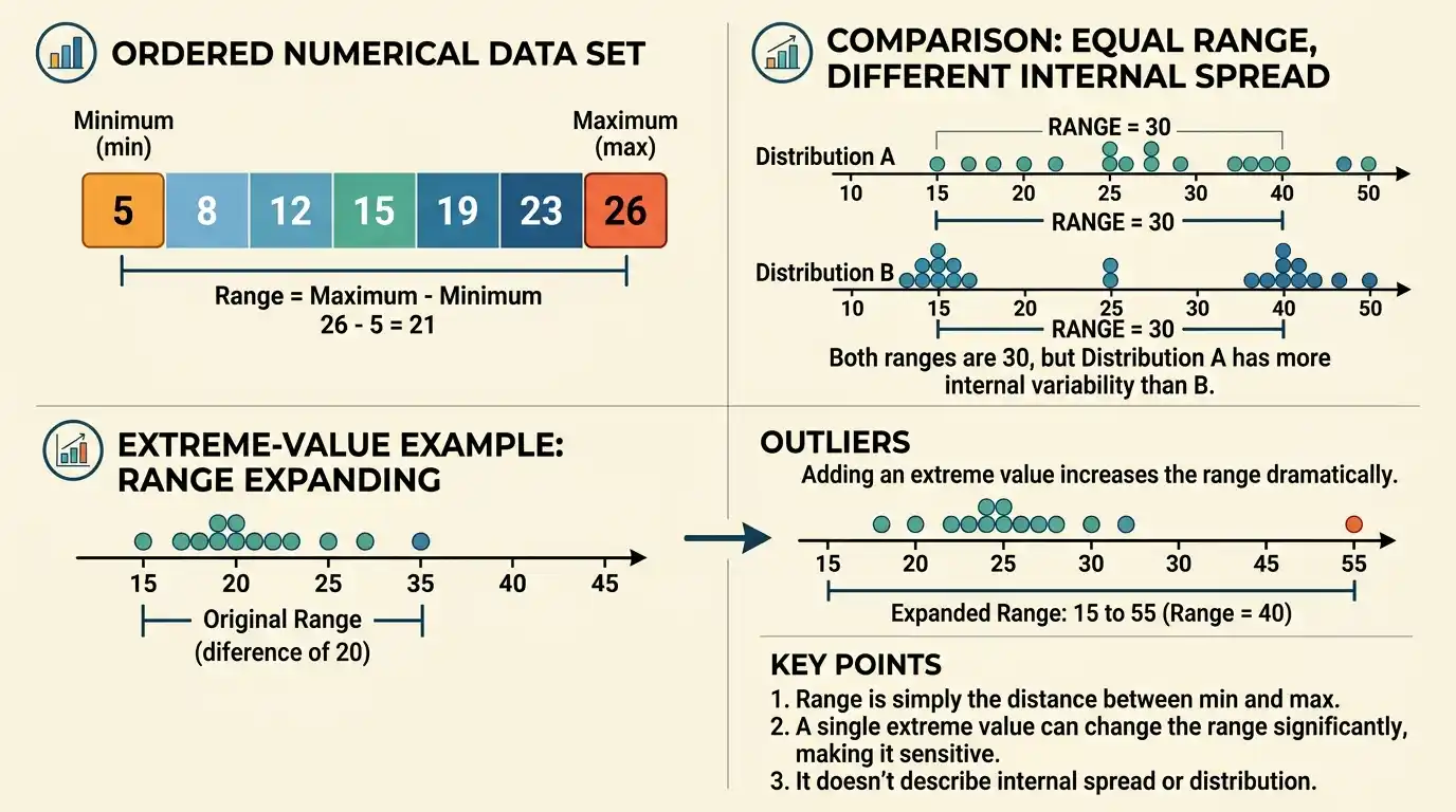
The range is one of the simplest measures of statistical dispersion, calculated as the difference between the largest and smallest values in a numerical data set. If the maximum observation is 25 and the minimum is 7, the range is 25 − 7 = 18, meaning the observed values span 18 units from one endpoint to the other. Because only the minimum and maximum are used, the range is exceptionally easy to calculate and provides an immediate description of total observed spread, but it ignores every value between those endpoints and can change dramatically when only one extreme observation changes. This sensitivity makes the range useful for quickly describing full span, checking measurement limits, comparing rough variability, and identifying unusually wide data sets, while also making it less stable than measures based on the central portion or all observations. A complete interpretation therefore considers the range alongside other summaries when the internal distribution, central spread, or influence of outliers matters.
The range is part of the broader toolkit of descriptive statistics within Statistics & Probability. It answers a narrow but important question—how far apart are the smallest and largest observed values?—without attempting to describe how observations are distributed between those endpoints.
What Is the Range?
The range is the numerical distance between the maximum and minimum values in a data set.
The formula is:
Range = Maximum − Minimum
Using symbols:
R = x_max − x_min
where:
- R = range
- x_max = largest observation
- x_min = smallest observation
The result has the same units as the original data.
If temperatures are measured in degrees Celsius, the range is measured in degrees Celsius. If distances are measured in kilometers, the range is measured in kilometers.
Simple Range Example
Consider:
3, 7, 10, 14, 18
The minimum is:
3
The maximum is:
18
Therefore:
Range = 18 − 3
= 15
So:
Range = 15
The observations span 15 units from the smallest to the largest value.
Why the Range Measures Spread
Suppose every observation in a data set is identical:
10, 10, 10, 10
Then:
Minimum = 10
Maximum = 10
Therefore:
Range = 10 − 10
= 0
A zero range indicates that the smallest and largest observations coincide, which can happen only when all observed values are equal.
As the distance between the endpoints grows, the range grows accordingly.
How to Calculate the Range Step by Step
The calculation requires only two observations.
First identify:
Minimum value
Then identify:
Maximum value
Subtract:
Maximum − Minimum
For unsorted data, it can be helpful to order the observations first, although sorting is not mathematically required if the minimum and maximum can already be identified correctly.
The result is always nonnegative for a nonempty numerical data set when maximum and minimum are defined conventionally.
Range Example With Unsorted Data
Consider:
22, 4, 15, 9, 31, 12
The smallest value is:
4
The largest value is:
31
Therefore:
R = 31 − 4
= 27
Sorting would produce:
4, 9, 12, 15, 22, 31
which makes the endpoints easy to see, but the final calculation is unchanged.
Range With Negative Numbers
Negative values do not require a different formula.
Consider:
−12, −7, −3, 2, 8
Minimum:
−12
Maximum:
8
Therefore:
Range = 8 − (−12)
= 8 + 12
= 20
A common error is forgetting that subtracting a negative number increases the result.
The span from −12 to 8 is 20 units.
Range When All Values Are Negative
Consider:
−20, −14, −9, −5
The maximum is:
−5
because −5 is numerically greater than −9, −14, and −20.
The minimum is:
−20
Therefore:
Range = −5 − (−20)
= 15
The range remains positive.
The signs of the endpoints do not determine the sign of the spread.
Range With Decimal Values
Consider:
1.25, 1.80, 2.10, 3.65
Maximum:
3.65
Minimum:
1.25
Therefore:
Range = 3.65 − 1.25
= 2.40
The range preserves the measurement scale and can contain decimals just like the original observations.
Range With One Observation
If a data set contains only:
12
then:
Minimum = 12
and:
Maximum = 12.
Therefore:
Range = 0.
This is mathematically valid for the observed data, although one observation provides essentially no information about the variability of a broader population.
Descriptive calculation and inferential usefulness are different issues.
Range With Two Observations
For:
8, 20
the range is:
20 − 8
= 12.
With only two observations, the range captures their entire separation.
There are no internal values to ignore.
As sample size grows, however, the range becomes an increasingly incomplete description because many different internal patterns can share the same endpoints.
The Range Uses Only Two Values
Suppose:
Data A = 0, 5, 5, 5, 10
and:
Data B = 0, 0, 0, 10, 10
Both have:
Minimum = 0
and:
Maximum = 10.
Therefore:
Range A = 10
Range B = 10.
Yet the observations are distributed very differently between the endpoints.
The range cannot distinguish those internal patterns because only the minimum and maximum enter its formula.
Same Range, Different Variability
Consider:
Data A = 0, 4, 5, 6, 10
and:
Data B = 0, 1, 2, 9, 10
Both have:
Range = 10.
However, Data A is concentrated around 5, while Data B places more observations near the ends.
A measure such as population variance would distinguish these patterns because it incorporates the distances of every observation from the mean.
The range cannot.
Range vs Variance
Range:
Maximum − Minimum
uses two observations.
Variance uses:
squared deviations from the mean
across all observations.
Consequently, two data sets can have the same range and different variances, or similar variances and different ranges.
Range measures endpoint separation.
Variance measures average squared dispersion.
Neither should be treated as a substitute for the other.
Range vs Sample Variance
When observed data are a sample from a larger population, sample variance summarizes squared spread around the sample mean, typically using:
s² = Σ(xᵢ − x̄)²/(n − 1)
under the standard unbiased estimator.
Range still uses:
x_max − x_min.
Sample variance therefore incorporates every observation and has a specific inferential role, whereas the sample range is fundamentally an endpoint statistic.
Both can describe sample dispersion, but they use very different information.
Range vs Standard Deviation
Standard deviation describes dispersion around the mean in the original measurement units.
Range describes total observed span.
Suppose:
Data A = 0, 5, 5, 5, 10
and:
Data B = 0, 0, 5, 10, 10.
Their ranges are both:
Their standard deviations differ because the internal positions differ.
Standard deviation therefore contains more information about typical dispersion around the center.
Range remains simpler and easier to compute.
Range vs Interquartile Range
The interquartile range is:
IQR = Q₃ − Q₁
and describes the span of the central half of the distribution.
Range is:
Maximum − Minimum
and describes the full observed span.
This distinction makes IQR considerably more resistant to extreme observations.
If one maximum becomes enormously larger, range changes immediately, while Q₁ and Q₃ may remain unchanged.
Thus, the two measures emphasize different regions of the distribution.
Range vs Median Absolute Deviation
Median absolute deviation summarizes typical absolute distance from the median, while range depends solely on the two endpoints.
Suppose:
1, 2, 3, 4, 1000
The range is:
1000 − 1
= 999.
Median:
Absolute deviations are:
2, 1, 0, 1, 997
so raw MAD is:
The range captures the huge endpoint span, while MAD describes the tightly concentrated central observations.
Both results are correct.
Range and Outliers
The range is extremely sensitive to outliers because the minimum and maximum determine it completely.
Suppose:
10, 11, 12, 13, 14
The range is:
14 − 10
= 4.
Now replace 14 with:
1,000.
The new range is:
1,000 − 10
= 990.
Only one observation changed, yet the range increased from 4 to 990.
This is why outlier detection can be important when interpreting an unexpectedly large span.
Does a Large Range Prove There Is an Outlier?
No.
A large range simply means the observed endpoints are far apart.
The distribution may genuinely cover a wide interval.
For example:
0, 20, 40, 60, 80, 100
has:
Range = 100.
No single observation appears isolated from the overall pattern.
Contrast this with:
0, 1, 2, 3, 4, 100
which also has:
Range = 100
but contains a highly separated upper observation.
Range alone cannot distinguish these cases.
Range and Sample Size
The observed range generally tends to increase as sample size grows because larger samples provide more opportunities to observe values farther into the population tails.
Suppose repeated samples are taken from the same continuous population.
A sample of:
n = 10
may miss rare tail values.
A sample of:
n = 100,000
is much more likely to include observations near more extreme population quantiles.
Therefore, raw ranges from samples of very different sizes should be compared cautiously.
A larger range does not automatically imply a more variable underlying population.
Sample Range as a Random Statistic
When data are sampled randomly, the minimum and maximum vary from sample to sample.
Therefore:
R = X_max − X_min
is itself a random statistic.
Two samples from the same population can have substantially different ranges, particularly when sample sizes are small.
This sampling instability is one reason the range is less commonly used than variance or IQR for formal inferential work.
Its simplicity is useful descriptively, but its dependence on extremes makes it noisy.
Population Range
If every member of a finite population is observed, population range is:
Population range = Population maximum − Population minimum.
For example, suppose the complete population is:
5, 8, 11, 13, 20
Then:
Minimum = 5
Maximum = 20
and:
Range = 15.
Because the entire finite population is known, this value describes its full span exactly.
There is no sampling uncertainty about the range of that specific defined population.
Sample Range vs Population Range
A sample may fail to contain the true population minimum or maximum.
Suppose a population spans:
0 to 100
but a sample happens to contain values only from:
18 to 83.
Then:
Sample range = 83 − 18
= 65
while:
Population range = 100 − 0
= 100.
Therefore, sample range generally should not be assumed to equal population range.
It often underestimates the total population span because the most extreme population members may not be sampled.
Range From a Frequency Table
When exact numerical values and their frequencies are known, range is easy to calculate from a frequency table.
Suppose:
| Value | Frequency |
|---|---|
| 2 | 4 |
| 5 | 7 |
| 9 | 3 |
| 15 | 2 |
The smallest value with positive frequency is:
The largest value with positive frequency is:
Therefore:
Range = 15 − 2
= 13.
The frequencies themselves do not affect the endpoint calculation once minimum and maximum values with positive counts are identified.
Relative Frequency and Range
A relative frequency table gives the proportion of observations associated with each value or interval rather than raw counts.
Suppose:
| Value | Relative Frequency |
|---|---|
| 10 | 0.20 |
| 20 | 0.50 |
| 30 | 0.30 |
All three values have positive relative frequency.
Therefore:
Minimum = 10
Maximum = 30
and:
Range = 20.
The size of each relative frequency does not alter the range as long as the endpoint values occur.
Range From Grouped Data
When data are grouped into intervals, the exact range may no longer be known.
Suppose nonempty classes are:
0–10
10–20
20–30
30–40.
A class-boundary approximation is:
Approximate range = 40 − 0
= 40.
However, the actual smallest observation could be:
4.7
and the largest:
36.2,
giving an exact raw-data range of:
31.5.
Grouped tables therefore often provide only an interval-based approximation to the true observed range.
Grouped Range Formula
For grouped data, a simple approximation is:
Approximate range = Upper boundary of highest nonempty class − Lower boundary of lowest nonempty class
This represents the entire possible span covered by the occupied classes.
It should not be described as the exact raw range unless observations are known to occur at those boundaries.
Grouping loses endpoint precision just as it loses information about exact internal values.
Open-Ended Classes
Suppose grouped data use:
Under 20
20–40
40–60
60+.
If observations occur in both open-ended classes, the exact range cannot be determined from the table because neither the true minimum nor maximum is specified.
Even one open-ended occupied endpoint class can prevent exact calculation.
Additional raw-data information is required.
Range and Mode
The mode identifies the most frequent value, whereas the range identifies endpoint separation.
Consider:
5, 5, 5, 6, 7, 100.
Mode:
Range:
100 − 5
= 95.
The mode shows concentration near 5.
The range shows that at least one observation lies far away.
Neither statistic alone describes the complete distribution.
Range and Distribution Shape
The range does not tell whether the data are:
- symmetric;
- skewed;
- unimodal;
- multimodal;
- uniformly distributed;
- clustered.
For example:
0, 2, 4, 6, 8, 10
and:
0, 0, 0, 10, 10, 10
both have:
Range = 10.
Their shapes are very different.
Range should therefore be interpreted strictly as endpoint spread.
Range and Gaps
A large internal gap does not affect the range if the endpoints stay the same.
Consider:
0, 1, 2, 8, 9, 10.
Range:
Now consider:
0, 4, 5, 5, 6, 10.
Range is also:
The first sample has a large central gap, while the second is concentrated centrally.
Range cannot reveal this distinction.
A distribution graph or frequency table is needed.
Range and Clusters
Suppose observations form two clusters:
1, 2, 3
and:
98, 99, 100.
The range is:
A single central summary of spread cannot reveal that the observations occupy two separated groups.
The large range indicates broad overall span but not why that span exists.
This is an important limitation whenever multimodality or subgroup structure is possible.
Range and Measurement Limits
Range can be useful for checking whether observations stay inside expected limits.
Suppose a manufacturing measurement is designed to remain between:
9.5 mm
and:
10.5 mm.
If recorded data have:
Minimum = 9.6
Maximum = 10.4
then:
Observed range = 0.8 mm.
Both endpoints lie inside the expected interval.
However, range alone does not tell how many observations are close to the limits.
Observed Range vs Specification Range
A specification interval might be:
9.5 to 10.5
with width:
1.0.
The observed data might span:
9.8 to 10.2
with range:
0.4.
These quantities should not be confused.
Specification range describes allowable or designed limits.
Observed range describes the endpoints actually present in the data.
A narrow observed range does not guarantee future observations will remain inside specification limits.
Range and Time-Series Data
For a time series over a fixed period, range can summarize the difference between the highest and lowest recorded values.
Suppose daily temperatures for one week have:
Minimum = 18°C
Maximum = 31°C.
Then:
Weekly temperature range = 13°C.
This provides a concise description of the week’s full observed temperature span.
It does not show when the maximum or minimum occurred or how temperatures changed between them.
Daily Range
Some contexts define a range within each observation period.
For example:
Daily temperature range = Daily maximum − Daily minimum.
If:
Maximum = 32°C
and:
Minimum = 19°C,
then:
Daily range = 13°C.
Repeated daily ranges can then themselves form a new data set for analysis.
The meaning of “range” should therefore specify the values whose endpoints are being compared.
Financial Price Range
A trading day’s observed price range might be calculated as:
High price − Low price.
If:
High = 105
Low = 97
then:
Range = 8.
This describes intraday span but does not reveal:
- opening price;
- closing price;
- trading volume;
- path between high and low.
Again, range summarizes endpoints rather than internal behavior.
Range and Rounding
Measurement rounding can alter observed endpoints.
Suppose true values are:
1.46 and 9.44.
Exact range:
9.44 − 1.46
= 7.98.
Rounded to whole numbers:
1 and 9
produce:
Range = 8.
The difference is small here, but coarse rounding can materially change the observed range when measurement precision is limited.
Calculations should use the most precise available values before final reporting.
Range and Missing Data
Missing values should not be interpreted as zero unless zero is genuinely observed.
Suppose valid data are:
10, 20, 30
with one missing record.
The observed valid range is:
30 − 10
= 20.
If the missing value is incorrectly coded as:
0,
the apparent range becomes:
30 − 0
= 30.
Incorrect missing-value coding can therefore distort endpoint statistics dramatically.
Range and Data-Entry Errors
The range can be an effective first-line data-quality diagnostic because extreme coding errors immediately affect the minimum or maximum.
Suppose typical measurements are:
10–20
but one value is accidentally entered as:
The range becomes enormous.
That does not tell us automatically that 1500 is wrong, but it signals that the endpoint deserves inspection.
Range is therefore useful in basic validation precisely because it is sensitive to extremes.
Unit Errors
Suppose most lengths are entered in centimeters:
160, 165, 172, 180
but one measurement of:
1.75 meters
is entered without conversion as:
1.75.
Then:
Minimum = 1.75
Maximum = 180
and:
Range = 178.25.
The unexpectedly large span may reveal the inconsistent unit.
Correcting:
1.75 m = 175 cm
would dramatically change the range without discarding a valid measurement.
Translation Property
Adding the same constant to every observation does not change the range.
Suppose:
Y = X + c.
Then:
max(Y) = max(X) + c
and:
min(Y) = min(X) + c.
Therefore:
Range(Y) = [max(X) + c] − [min(X) + c]
= max(X) − min(X)
= Range(X).
A uniform shift changes location but not spread.
Translation Example
Suppose:
X = 2, 5, 9.
Range:
9 − 2
= 7.
Add:
100
to every observation:
Y = 102, 105, 109.
Range:
109 − 102
= 7.
The endpoints shift by the same amount, so their separation remains unchanged.
Scaling Property
If every observation is multiplied by a constant a:
Y = aX,
then:
Range(Y) = |a|Range(X).
The absolute value is necessary because a negative multiplier reverses the ordering of minimum and maximum.
For positive a, the interval simply stretches or contracts by the factor a.
Positive Scaling Example
Suppose:
X = 2, 5, 9
with:
Range = 7.
Multiply every observation by:
Then:
Y = 6, 15, 27.
Range:
27 − 6
= 21.
And:
3 × 7 = 21.
Therefore:
Range(3X) = 3Range(X).
Negative Scaling Example
Suppose:
X = 2, 5, 9
and multiply by:
−2.
Then:
Y = −4, −10, −18.
Ordered:
−18, −10, −4.
Range:
−4 − (−18)
= 14.
The original range was:
Therefore:
Range(−2X) = 2(7)
= 14.
The sign reversal changes order but not absolute endpoint distance.
General Linear Transformation
For:
Y = aX + b
the range satisfies:
Range(Y) = |a|Range(X).
The constant:
b
does not matter because it shifts every observation equally.
The scale factor:
a
changes distances by:
|a|.
This property makes range easy to transform under ordinary changes of measurement units.
Unit Conversion Example
Suppose temperatures measured on a scale differ by:
10°C
from minimum to maximum.
Converting temperature differences to Fahrenheit multiplies the difference by:
1.8.
Therefore:
Fahrenheit range = 1.8(10)
= 18°F.
The additive 32 used in the Celsius-to-Fahrenheit conversion does not affect the range because translation cancels.
Range Is Not a Ratio
Suppose:
Minimum = 10
Maximum = 20.
Range:
This does not mean the maximum is “10 times” the minimum.
A range is a difference, not a ratio.
If proportional spread matters, another measure is required.
The same numerical range can represent very different relative variation depending on the overall measurement scale.
Relative Importance of the Same Range
Compare:
Data A spans 1 to 11
and:
Data B spans 10,000 to 10,010.
Both ranges are:
Relative to the magnitudes involved, however, the first span is much larger.
Therefore, raw range is an absolute dispersion measure.
It should not automatically be used for proportional comparisons across vastly different scales.
Range and Bounded Variables
Some variables have natural limits.
For probabilities:
0 ≤ p ≤ 1.
The largest possible theoretical span is:
1 − 0
= 1.
For percentages constrained between 0% and 100%, the largest possible range is:
100 percentage points.
Knowing the variable’s support can provide context for whether an observed range is narrow or broad.
Observed Range vs Theoretical Range
A variable can have a theoretical range much larger than the observed range.
Suppose exam scores can vary from:
0 to 100.
The theoretical possible range is:
If one class records:
Minimum = 62
Maximum = 91,
its observed range is:
The two concepts should not be confused.
One describes the allowable scale, while the other describes values actually observed.
Range of a Probability Distribution
For a random variable with bounded support:
a ≤ X ≤ b,
the support span is:
b − a.
For a uniform distribution on:
[a, b],
this interval width is often central to the model.
For unbounded distributions such as the normal distribution, the theoretical support extends indefinitely, so there is no finite population support range even though every finite sample has a finite observed range.
Normal Distribution and Range
A normal random variable has support:
(−∞, ∞).
Therefore, its theoretical range is infinite.
However, any finite sample from a normal distribution contains a finite minimum and maximum.
Thus:
finite sample range
does not imply:
bounded population support.
This distinction is important when using observed endpoints to infer possible future values.
Range and Order Statistics
The sample minimum and maximum are order statistics.
If sorted observations are:
X_(1) ≤ X_(2) ≤ … ≤ X_(n),
then:
Minimum = X_(1)
and:
Maximum = X_(n).
Therefore:
Sample range = X_(n) − X_(1).
This notation emphasizes that range depends entirely on the two extreme order statistics.
Why Range Becomes More Stable With More Data—But Also Larger
As sample size grows, the observed minimum and maximum can become more representative of the population tails, reducing some random fluctuation relative to a fixed sample size.
At the same time, larger samples typically extend farther toward the tails, so expected range can increase.
These two effects are compatible.
The statistic may become more predictable for a given n while its expected numerical value changes with n.
This is why range comparisons should account for sample size.
Range in Quality Control
In some process-monitoring settings, ranges of small subgroups are used as quick measures of within-subgroup variation.
For a subgroup:
R = max − min.
Repeated subgroup ranges can then be summarized over time.
Because the range is simple and fast to calculate, it has historical importance in certain control-chart methods.
However, such procedures use carefully defined subgroup sizes and constants; an ordinary raw range should not be treated as a universal process-capability measure.
Why Range Can Be Useful Despite Its Limitations
The range survives as a useful statistic because it is immediate and intuitive.
It can quickly answer:
- What are the endpoints?
- How wide is the observed span?
- Did the process exceed expected limits?
- Is one data set obviously broader than another?
- Could there be an extreme recording problem?
These are practical questions.
The limitation is that the range cannot explain what happens between the endpoints.
Range and Robustness
Range is one of the least robust common measures of dispersion.
Changing a single endpoint can change the statistic by an arbitrarily large amount.
For example:
1, 2, 3, 4, 5
has range:
Replace 5 with:
1,000,000.
The range becomes:
999,999.
Therefore, range has essentially no resistance to extreme endpoint contamination.
This sensitivity must be considered whenever measurement errors or outliers are plausible.
Full Worked Example
Consider:
14, 7, 22, 19, 11, 30, 5, 18
Step 1: Identify the Minimum
Minimum = 5
Step 2: Identify the Maximum
Maximum = 30
Step 3: Subtract
Range = 30 − 5
= 25
Therefore:
Range = 25
The observed data span 25 units from smallest to largest.
Verify by Sorting
Sort the observations:
5, 7, 11, 14, 18, 19, 22, 30
The endpoints are clearly:
5 and 30.
Therefore:
R = 30 − 5
= 25.
All six observations between those endpoints have no effect on the numerical range.
They matter for other measures of center and spread, but not for this calculation.
Worked Example With Negative and Positive Values
Consider:
−25, −8, −3, 4, 17, 31
Minimum:
−25
Maximum:
31
Therefore:
Range = 31 − (−25)
= 56.
The observed values span:
56 units.
A useful check is to think of the interval as extending 25 units from −25 to 0 and another 31 units from 0 to 31:
25 + 31 = 56.
Worked Frequency-Table Example
Suppose:
| Score | Frequency |
|---|---|
| 40 | 2 |
| 50 | 8 |
| 60 | 12 |
| 70 | 6 |
| 80 | 1 |
The smallest score occurring is:
The largest is:
Therefore:
Range = 80 − 40
= 40.
The fact that score 60 occurs twelve times does not affect the range.
Only the endpoints matter.
Worked Grouped-Data Example
Suppose the nonempty intervals are:
| Interval | Frequency |
|---|---|
| 10–20 | 4 |
| 20–30 | 8 |
| 30–40 | 12 |
| 40–50 | 5 |
Using class boundaries:
Approximate range = 50 − 10
= 40.
However, if the actual minimum is:
13
and actual maximum:
47,
then the exact raw range would be:
Because those exact endpoints are not visible in the grouped table, 40 should be described as the class-boundary span or approximate range.
Comparing Two Data Sets
Consider:
A = 10, 11, 12, 13, 14
and:
B = 2, 10, 11, 12, 22.
For A:
Range = 14 − 10
= 4.
For B:
Range = 22 − 2
= 20.
Thus, B has a much wider observed endpoint span.
However, three of B’s five observations remain close to 10–12, so the large range is driven primarily by the endpoints.
This is why internal spread should be inspected before interpreting the difference as general variability.
Common Range Mistakes
A common mistake is subtracting the first listed value from the last listed value without first checking whether those observations are actually the minimum and maximum.
Another mistake is calculating:
Minimum − Maximum,
which gives a negative number rather than the conventional nonnegative range.
Negative-value data can also create sign errors, particularly when subtracting a negative minimum.
Analysts sometimes treat a wide range as proof that every observation is widely dispersed even though one extreme point may account for nearly all of the span.
Another mistake is comparing ranges from dramatically different sample sizes without considering that larger samples naturally have more opportunities to contain extreme observations.
For grouped data, using outer class boundaries and calling the result an exact raw range is also misleading.
Finally, range should not be confused with IQR, standard deviation, variance, or a permitted specification interval.
How to Calculate Range Correctly
Begin with valid numerical observations and exclude missing-value codes that are not genuine measurements.
Identify the true minimum:
x_min.
Identify the true maximum:
x_max.
Then calculate:
R = x_max − x_min.
Keep the original measurement units.
If the data are grouped, distinguish the approximate class span from the unknown exact raw range.
When the result is unexpectedly large, examine whether the endpoint represents a valid extreme observation, an expected tail value, or a data-quality problem.
When to Use the Range
Range is particularly useful when:
- a quick measure of total spread is needed;
- minimum and maximum are substantively important;
- checking measurement or operational limits;
- data sets are small and transparent;
- endpoint variation itself is meaningful;
- simple descriptive summaries are required.
It is often useful as part of an initial data review.
Its simplicity makes unusual endpoint behavior easy to detect.
When Range Alone Is Not Enough
Range should be supplemented when:
- outliers are present;
- sample sizes differ substantially;
- internal distribution shape matters;
- typical spread is more important than endpoint spread;
- data are strongly skewed;
- grouped intervals obscure exact endpoints.
Measures such as variance, standard deviation, IQR, and MAD provide different views of dispersion.
Using several complementary summaries can reveal whether a large range represents general spread or merely a few extreme observations.
How to Report the Range
A concise report can state:
“Values ranged from 5 to 30, giving a range of 25 units.”
This is often clearer than reporting:
“Range = 25”
alone because it preserves both endpoints.
For grouped data:
“The occupied classes extended from 10–20 through 40–50, giving an approximate class-boundary span of 40 units.”
When one unusual observation dominates the span, mention that context rather than allowing the one-number statistic to imply uniform dispersion.
Frequently Asked Questions About Range
What is the range?
The range is the difference between the maximum and minimum observations.
What is the formula?
Range = Maximum − Minimum
What symbol can represent range?
A common simple notation is:
R = x_max − x_min.
What does the range measure?
It measures the total observed span of numerical data.
What is the range of 3, 7, 10, and 15?
15 − 3 = 12.
Can range be negative?
Not under the standard maximum-minus-minimum definition.
What is the minimum possible range?
When is the range zero?
When all observed values are identical.
Does range use every observation?
No. It uses only the minimum and maximum.
Does range have the same units as the data?
Yes.
Is range measured in squared units?
No. Variance uses squared units; range remains in the original units.
Can range be calculated with negative values?
Yes.
What is the range of −10 to 5?
5 − (−10) = 15.
Can range be a decimal?
Yes.
Can a one-value data set have a range?
Yes:
Range = 0.
Is range the same as variance?
No.
How does variance differ?
Variance uses squared deviations of all observations from the mean.
Is range the same as standard deviation?
No.
How does standard deviation differ?
Standard deviation summarizes mean-centered dispersion using all observations.
Is range the same as IQR?
No.
What is IQR?
Q₃ − Q₁,
which describes the middle half of the distribution.
Which is more sensitive to outliers, range or IQR?
Range.
Is range robust?
No. It is extremely sensitive to endpoint outliers.
Can one outlier change the range dramatically?
Yes.
Does a large range prove there is an outlier?
No.
Why not?
The population may legitimately occupy a wide interval.
Can two data sets have the same range but different variance?
Yes.
Can two data sets have the same range but different shapes?
Yes.
Does range reveal skewness?
No.
Does range reveal multimodality?
No.
Does range reveal gaps?
No.
Does range identify the most common value?
No. That is the role of the mode.
Can range be calculated from a frequency table?
Yes, when exact endpoint values with positive frequency are known.
Do frequencies affect the range?
Not directly. Only the smallest and largest values occurring matter.
Can range be calculated from relative frequencies?
Yes, if exact values associated with positive relative frequencies are known.
Can grouped data provide an exact range?
Usually not unless the exact raw minimum and maximum are also known.
How is grouped range approximated?
A common approximation is:
Highest occupied class upper boundary − Lowest occupied class lower boundary.
What happens with open-ended classes?
The exact range may be impossible to determine.
Does adding 10 to every observation change the range?
No.
What is the translation property?
Range(X + c) = Range(X).
What happens if every observation is doubled?
The range doubles.
What is the scaling property?
Range(aX) = |a|Range(X).
Why is the absolute value used?
A negative multiplier reverses order but distances remain nonnegative.
Can the sample range equal the population range?
Yes, if the sample happens to contain the population minimum and maximum.
Does it always?
No.
Why does sample size affect range?
Larger samples have more opportunities to include extreme population values.
Can range be used to estimate variability?
It provides a rough measure of endpoint spread but is generally less stable than measures using more observations.
Is range useful for quality control?
It can be useful in defined subgroup-based procedures and as a quick endpoint check.
Is the observed range the same as specification width?
No.
What is observed range?
The span between actual sample or population endpoints.
What is specification width?
The span between predetermined allowable limits.
Can missing-value coding affect range?
Yes, dramatically if a missing code is treated as a real extreme numerical value.
Can unit errors affect range?
Yes. Inconsistent units can create artificial extremes.
Should an extreme endpoint always be deleted?
No.
What should happen instead?
Verify whether it is correctly recorded, belongs to the target data, and represents a legitimate extreme observation.
What is the main advantage of range?
It gives an immediate, intuitive measure of the full observed numerical span with almost no calculation.
What is its main limitation?
It uses only two observations, making it highly sensitive to extremes and unable to describe how data are distributed between the minimum and maximum.
What is the most important rule when using the range?
Identify the true minimum and maximum, subtract the minimum from the maximum, and interpret the result strictly as endpoint spread, not as a complete measure of the distribution’s typical variability.