The median is a measure of central tendency that identifies the middle position of an ordered numerical data set, dividing the observations so that roughly half lie at or below it and half lie at or above it. Unlike the arithmetic mean, which depends on the numerical magnitude of every observation, the median depends primarily on rank, making it comparatively resistant to unusually large or small values. For an odd number of observations, the median is the single value occupying the central ordered position, while for an even number of observations it is conventionally calculated as the arithmetic mean of the two central values. This rank-based behavior makes the median particularly useful for skewed distributions, income data, property values, waiting times, and other situations where a few extreme observations can pull an arithmetic average away from the typical center. However, the median also discards some magnitude information because changing observations substantially without changing their positions around the center can leave the median unchanged.
Within descriptive statistics and the broader Statistics & Probability framework, the median is one of the most important positional summaries because it connects central tendency with quartiles, percentiles, robust spread, and ordered-data analysis. It is simple to calculate from raw observations, can be located efficiently from frequency tables, and can be estimated from grouped data when exact individual measurements are unavailable.
What Is the Median?
The median is the central value of a data set after the observations have been arranged in numerical order.
Suppose the ordered values are:
2, 4, 7, 9, 12
The central observation is:
7
so:
Median = 7
There are two observations below 7 and two above it.
This illustrates the central rank property of the median.
Its interpretation is positional rather than additive.
Median Formula for an Odd Number of Observations
For:
n = odd
the median position is commonly written:
Median position = (n + 1)/2
after the observations are sorted.
Suppose:
n = 9
Then:
Median position = (9 + 1)/2
= 5
The fifth ordered observation is the median.
The formula gives a position, not necessarily the numerical median directly.
The value occupying that position must then be identified.
Odd-Sample Example
Consider:
14, 3, 9, 20, 7, 11, 5
First sort the values:
3, 5, 7, 9, 11, 14, 20
There are:
n = 7
observations.
Therefore:
Median position = (7 + 1)/2
= 4
The fourth value is:
9
so:
Median = 9
Sorting is essential because the fourth value in the original unsorted sequence would not represent the central rank.
Median Formula for an Even Number of Observations
For:
n = even
there is no single observation occupying the unique center.
The two middle positions are:
n/2
and:
n/2 + 1
The ordinary numerical median is their arithmetic average:
Median = [x_(n/2) + x_(n/2+1)]/2
where the x-values represent sorted observations.
Suppose:
n = 8.
The middle positions are:
4th and 5th.
Those two values determine the median.
Even-Sample Example
Consider:
2, 5, 7, 10, 12, 15, 18, 25
There are:
n = 8.
The fourth value is:
10
and the fifth is:
Therefore:
Median = (10 + 12)/2
= 22/2
= 11
Notice that:
11
does not appear in the original data.
The median can therefore be a value between observations when n is even.
Why the Data Must Be Sorted
The median describes rank, so the original input order is irrelevant.
Suppose the data are:
100, 3, 8, 20, 6
Reading the third entry directly would give:
8
but first sort:
3, 6, 8, 20, 100.
In this case the central value still happens to be 8.
However, that agreement is accidental.
With a different original arrangement, the middle-listed observation could be completely unrelated to the median.
Always sort before identifying central positions.
Median as the 50th Percentile
The median corresponds to the central percentile position:
50th percentile.
It is also commonly denoted:
Q₂
because it is the second quartile.
Conceptually, approximately half of observations lie at or below the median and approximately half lie at or above it.
Repeated observations can make more than half of the sample equal to the median, so the interpretation should not be stated as though exactly 50% must be strictly smaller and exactly 50% strictly larger.
Rank relationships allow equality.
Median and Quartiles
The median divides an ordered distribution into lower and upper halves.
Quartiles then divide the data more finely:
Q₁ ≈ 25th percentile
Q₂ = Median
Q₃ ≈ 75th percentile.
Together, Q₁, median, and Q₃ describe the central rank structure of the distribution.
The distance:
Q₃ − Q₁
is the interquartile range.
Thus, the median is central not only as a measure of location but also within the broader quartile framework.
Median vs Arithmetic Mean
The arithmetic mean is based on:
x̄ = Σxᵢ/n.
The median is based on ordered position.
Consider:
1, 2, 3, 4, 100
The mean is:
(1 + 2 + 3 + 4 + 100)/5
= 110/5
= 22
while:
Median = 3.
The large observation 100 pulls the mean far above most of the sample.
The median remains anchored at the central rank.
This resistance to extreme magnitudes is one of its major advantages.
Why the Median Is Robust
Suppose:
10, 11, 12, 13, 14
The median is:
Now replace the largest observation:
14
with:
1,000,000.
The sorted data become:
10, 11, 12, 13, 1,000,000
and:
Median = 12.
The arithmetic mean changes enormously, but the median is unchanged.
As long as the central rank does not move, extreme magnitude changes can have no effect on the median.
Breakdown Resistance
The median has strong robustness because a substantial fraction of observations must be moved across the center before the statistic can be driven arbitrarily far.
Informally, nearly half the sample can become extremely contaminated while the central order statistic can still remain bounded by the uncontaminated observations.
This is very different from the arithmetic mean, where a single arbitrarily large value can make the average arbitrarily large.
That robustness is one reason the median is widely used when tail contamination is plausible.
Median and Skewed Data
For a strongly right-skewed distribution, the median often provides a more representative central location than the mean.
Consider household incomes:
30, 32, 35, 36, 40, 42, 500
The median is:
36
while the mean is:
715/7
≈ 102.14.
The mean is numerically valid, but one extremely large income makes it far larger than the values experienced by most observations.
The median better reflects the central ranked household in this particular sample.
Median in a Right-Skewed Distribution
In many right-skewed distributions:
Mean > Median.
Large upper-tail values pull the mean upward while the median remains tied to the 50th-percentile position.
This relationship is common but is not the mathematical definition of right skewness.
Distribution shape should be examined directly rather than inferred from one inequality alone.
A histogram can help show whether the sample actually has a long upper tail, several modes, gaps, or another structure.
Median in a Left-Skewed Distribution
For many left-skewed distributions:
Mean < Median.
Small lower-tail observations pull the arithmetic mean downward.
The median remains centered by rank.
For example:
−100, 10, 12, 14, 16
has:
Median = 12
while:
Mean = −48/5
= −9.6.
The extreme lower observation causes the two measures to differ dramatically.
Again, the relationship is descriptive rather than universal.
Median in a Symmetric Distribution
In a perfectly symmetric distribution, the population mean and median often coincide when both are well-defined.
For a symmetric sample such as:
1, 3, 5, 7, 9
we have:
Median = 5
and:
Mean = 5.
This agreement can make either statistic a reasonable measure of center.
However, symmetry alone does not imply normality.
Many distributions are symmetric without being bell-shaped or normally distributed.
Median and Mode
The mode is the most frequently occurring value, while the median is the central ranked value.
Consider:
1, 2, 2, 2, 10, 20, 30
Then:
Mode = 2
while:
Median = 2.
In another sample:
1, 1, 2, 3, 4, 5, 6
we have:
Mode = 1
but:
Median = 3.
The two measures answer different questions: one identifies frequency concentration, while the other identifies central order.
Median With Repeated Values
Repeated values are handled naturally.
Consider:
2, 2, 2, 5, 8, 9, 10
There are:
n = 7
observations.
The fourth value is:
5
so:
Median = 5.
Now consider:
2, 2, 5, 5, 5, 9, 10.
The median is again:
Several observations can equal the median without affecting its interpretation.
Median Can Equal the Minimum
Suppose:
1, 1, 1, 1, 10
The central value is:
Therefore:
Median = Minimum = 1.
Likewise, the median can equal the maximum when many observations take the upper endpoint.
This is perfectly valid.
The median need only satisfy its positional definition; it does not have to lie strictly between the minimum and maximum.
Median With Negative Values
Negative numbers require no special treatment.
Consider:
−20, −10, −4, 2, 8
The middle observation is:
−4.
Therefore:
Median = −4.
For:
−20, −10, −4, 2
the two middle values are:
−10 and −4.
Thus:
Median = (−10 + −4)/2
= −14/2
= −7.
The same sorting and position rules apply.
Median With Decimal Values
The median can be a decimal whether or not the original observations contain decimals.
Consider:
2, 5, 8, 11
The two central observations are:
5 and 8.
Therefore:
Median = (5 + 8)/2
= 6.5.
There is no requirement that the median itself be observed.
It is an ordered-data summary.
Median From a Frequency Table
A frequency table can locate the median without expanding every repeated observation individually.
Suppose:
| Value | Frequency |
|---|---|
| 1 | 3 |
| 2 | 4 |
| 3 | 5 |
| 4 | 2 |
Total frequency is:
n = 3 + 4 + 5 + 2
= 14.
The central positions are:
7th and 8th.
We can locate those positions by accumulating frequencies.
Frequency-Table Median Example
The cumulative counts are:
Value 1 → positions 1–3
Value 2 → positions 4–7
Value 3 → positions 8–12
Value 4 → positions 13–14
Therefore:
7th observation = 2
and:
8th observation = 3.
Thus:
Median = (2 + 3)/2
= 2.5
The full expanded list is unnecessary.
Rank locations can be found directly from frequencies.
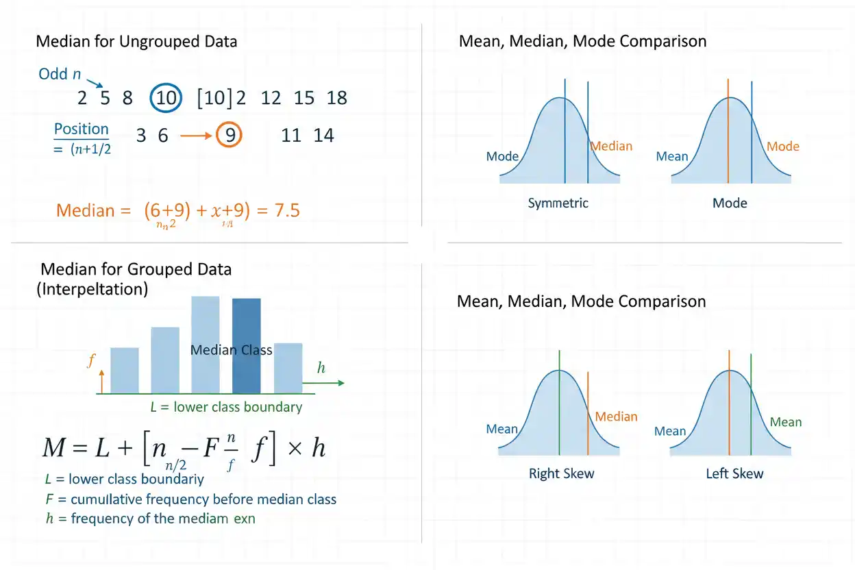
Median From Grouped Data
When only grouped intervals are known, the exact median of the raw observations is usually unavailable.
Instead, one identifies the median class and interpolates within that class.
A common formula is:
Median ≈ L + [(n/2 − F_prev)/f_m]h
where:
- L = lower class boundary of the median class
- n = total frequency
- F_prev = cumulative frequency before the median class
- f_m = frequency of the median class
- h = class width
This formula assumes observations are distributed approximately uniformly through the median class.
Grouped Median Example
Suppose:
| Class | Frequency | Cumulative Frequency |
|---|---|---|
| 0–10 | 4 | 4 |
| 10–20 | 6 | 10 |
| 20–30 | 10 | 20 |
| 30–40 | 8 | 28 |
| 40–50 | 2 | 30 |
Total:
n = 30.
The central position is approximately:
n/2 = 15.
The first cumulative frequency reaching or exceeding 15 is:
20
in the:
20–30
class.
Therefore, 20–30 is the median class.
Calculate the Grouped Median
Use:
L = 20
F_prev = 10
f_m = 10
h = 10.
Then:
Median ≈ 20 + (15 − 10)/10
= 20 + (5/10)(10)
= 20 + 5
= 25.
Therefore:
Grouped median ≈ 25.
This is an estimate because the original observations within 20–30 are unknown.
Why Grouped Median Is Approximate
Suppose ten observations lie in:
20–30.
They could be concentrated near:
20
or near:
The grouped table does not reveal their exact locations.
Interpolation assumes a regular spread across the interval for estimation purposes.
If that assumption is poor, the estimated median can differ from the actual raw-data median.
Narrow classes generally reduce this information loss.
Median Class
The median class is the interval containing the central cumulative-frequency position.
For:
n = 80,
the central location is around:
Find the first cumulative frequency that reaches or exceeds:
That class is the median class.
The median class is not itself the median value.
A numerical estimate within the class requires interpolation or access to the original observations.
Median for Ordinal Data
The median can be meaningful for ordinal variables because ordinal categories possess an order.
Suppose responses are:
Poor
Fair
Good
Very Good
Excellent.
If the central ranked response is:
Good,
then Good can be described as the median category.
Unlike the arithmetic mean, the calculation does not require assuming equal numerical spacing between categories.
This makes the median useful for many ordered ratings.
Median for Nominal Data
The median is generally not meaningful for nominal categories that lack an intrinsic order.
Examples include:
Red
Blue
Green.
One can count the most common category and identify a mode, but there is no natural central rank because:
Red < Blue < Green
has no inherent quantitative or ordinal meaning.
Artificially assigning numbers does not create a meaningful median unless the coding reflects a genuine order.
Median for Binary Data
Binary variables have two ordered numerical outcomes when coded naturally as:
0 and 1.
If fewer than half the observations are 1, the median is often:
If more than half are 1:
Median = 1.
For an even sample with exactly half zeros and half ones, the conventional numerical median becomes:
(0 + 1)/2
= 0.5.
That value is not an observed category, so interpretation should recognize the coding structure.
Weighted Median
A weighted median generalizes the ordinary median by allowing observations to represent unequal amounts.
The weighted median is a value at which cumulative weight reaches at least half the total weight, with definitions varying slightly in tie cases.
Suppose:
| Value | Weight |
|---|---|
| 10 | 1 |
| 20 | 2 |
| 30 | 7 |
Total weight is:
Half the total weight is:
Cumulative weight reaches:
1 at 10
3 at 20
10 at 30.
Therefore:
Weighted median = 30.
Why Weighted Median Can Differ From Ordinary Median
For the values:
10, 20, 30
the ordinary median is:
But with weights:
1, 2, 7
the weighted median becomes:
The largest weight places most represented mass at 30.
Weighted medians are useful when observations represent different population counts, exposures, or importance levels.
The weights must have a meaningful interpretation rather than being chosen merely to shift the answer.
Median and Absolute Deviations
The median has an important optimization property.
For observed values xᵢ, a median minimizes:
Σ|xᵢ − c|
over possible central locations c.
In other words, the median minimizes total absolute deviation.
The arithmetic mean has a parallel squared-error property:
x̄ minimizes Σ(xᵢ − c)².
This difference helps explain why the median is associated naturally with absolute-error methods and robustness, while the mean is associated with least-squares methods.
Absolute-Deviation Example
Consider:
1, 2, 10.
The median is:
Total absolute deviation around 2 is:
|1−2| + |2−2| + |10−2|
= 1 + 0 + 8
= 9.
Try center:
c = 4.
Then:
|1−4| + |2−4| + |10−4|
= 3 + 2 + 6
= 11.
The median produces the smaller total absolute deviation.
Median Absolute Deviation
The median absolute deviation builds directly on the median as a robust measure of spread.
First find:
Median(x)
Then calculate absolute deviations:
|xᵢ − Median(x)|.
The median of those deviations is:
MAD = Median(|xᵢ − Median(x)|).
Because both steps use medians rather than squared deviations, MAD remains comparatively resistant to extreme observations.
It provides a natural robust companion to the median as a measure of center.
Median and Kurtosis
Kurtosis reacts strongly to extreme observations because it involves fourth-power deviations from the mean.
The median behaves almost oppositely.
A single enormous value can radically increase sample kurtosis while leaving the median completely unchanged.
This contrast illustrates why no single statistic can fully describe a data set.
The median provides robust central location.
Kurtosis describes extreme standardized deviation behavior.
Both can be useful for heavily tailed distributions, but they answer different questions.
Median and Margin of Error
A margin of error describes inferential uncertainty around an estimated population quantity, whereas the sample median itself is a descriptive point estimate.
The ordinary mean formula:
z*σ/√n
should not automatically be used for a median because the median has a different sampling distribution.
Confidence intervals for a population median can instead be constructed using order statistics, quantile theory, or bootstrap methods.
Thus, a median can have uncertainty just like a mean, but its inferential formula must be appropriate to its rank-based nature.
Median of a Population vs Median of a Sample
A population median is the central quantile of the entire population distribution.
A sample median is calculated from observed sample values and serves as an estimator of the population median.
Different random samples usually produce different sample medians.
Therefore:
Sample median ≠ guaranteed population median.
Larger representative samples generally provide more stable information about the population center, though the exact uncertainty depends on the distribution around its median.
Sampling Distribution of the Median
The sample median is a random statistic.
Across repeated samples, its variability depends strongly on how much probability density lies near the population median.
When observations are densely concentrated around the median, small ranking changes produce relatively small numerical changes.
When the population distribution is sparse or flat near its median, the sample median can vary more widely.
Thus, sample size alone does not determine median precision.
Local distribution shape matters too.
Approximate Standard Error of a Median
For a sufficiently regular continuous distribution with density f evaluated at population median m, the large-sample variance of the sample median is approximately:
Var(Median) ≈ 1/[4n f(m)²]
so:
SE(Median) ≈ 1/[2√n f(m)].
This formula shows explicitly that median precision depends on the density near the center.
A high f(m) gives a smaller standard error.
A low f(m) produces greater uncertainty.
The result is asymptotic and should not be applied mechanically to every distribution or small sample.
Normal-Distribution Median Precision
For a normal population:
Mean = Median = μ.
Using the normal density at μ, the asymptotic standard error of the sample median is approximately:
SE(Median) ≈ σ√[π/(2n)].
By comparison:
SE(Mean) = σ/√n.
Therefore, under exact normality, the sample mean is more statistically efficient for estimating μ.
The median sacrifices some efficiency in this ideal setting in exchange for much greater resistance to contamination and extreme observations.
Relative Efficiency Under Normality
The asymptotic efficiency of the sample median relative to the sample mean for normal data is:
2/π
≈ 0.637.
This means the median requires more observations than the mean to achieve the same asymptotic variance when the population is exactly normal.
However, this does not imply the mean is always preferable.
When the population has heavy tails or contamination, the median’s robustness can outweigh its lower normal-theory efficiency.
Median and Outliers
The median is resistant to isolated outliers, but it is not completely unaffected by all contamination.
Suppose:
1, 2, 3, 4, 5.
Median:
Replacing 5 with 5000 leaves the median unchanged.
However, if several observations are changed so that they cross the center of the ordered sample, the median can move.
Robust does not mean immutable.
It means unusually large magnitudes have limited influence unless enough ranks are affected.
Example With Multiple Extreme Values
Start with:
1, 2, 3, 4, 5, 6, 7
Median:
Replace the two largest values:
6, 7
with:
1,000, 10,000.
The median remains:
Replace four of the seven values with huge numbers, however, and the central rank can move dramatically.
The median’s resistance comes from ordering, not from ignoring data entirely.
Median and Missing Data
Missing values should not be automatically treated as zero.
Suppose observed valid data are:
10, 20, 30.
Then:
Median = 20.
If one missing observation is incorrectly coded as:
0,
the data become:
0, 10, 20, 30
and:
Median = 15.
The result changes even though no real zero was observed.
Missing-data handling must therefore precede median calculation.
Median and Censoring
Censoring can limit exact median estimation.
Suppose measurements above:
100
are recorded only as:
100+.
If the median lies well below 100, this may not affect its numerical value.
If at least half the observations are censored above 100, however, the exact median may be unknown beyond that threshold.
The rank-based nature of the median can make it relatively robust to tail censoring, but not when censoring reaches the center of the distribution.
Median and Truncation
Truncation removes observations outside a defined range from the observed sample.
For example, if all values below:
10
are excluded by design, the median of the observed data describes the truncated population rather than the original full population.
It can be perfectly calculated yet answer a different question from the intended one.
As with every descriptive statistic, interpretation depends on how observations entered the data set.
Median and Monotonic Transformations
For a strictly increasing transformation g:
Median[g(X)] = g[Median(X)]
under the usual quantile interpretation.
For example, if:
Y = 10X + 5,
then:
Median(Y) = 10Median(X) + 5.
This property is stronger than what holds for many arithmetic summaries.
Because strictly increasing transformations preserve order, the central rank transforms naturally.
Log Transformation Example
Suppose positive data have:
Median(X) = 20.
Let:
Y = ln(X).
Because logarithm is strictly increasing:
Median(Y) = ln(20)
under the corresponding quantile definition.
Conversely:
Median(X) = exp[Median(ln X)].
This property makes medians convenient when moving between raw and logarithmic scales.
Decreasing Transformations
If g is strictly decreasing, the order reverses.
However, the central 50th-percentile location still transforms consistently:
Median[g(X)] = g[Median(X)]
under standard continuous-distribution conditions.
For a finite sample, care with even-sample averaging can matter because averaging and nonlinear transformation need not commute.
For odd samples with one unique central observation, the rank transformation is especially straightforward.
Adding a Constant
If every observation increases by c:
yᵢ = xᵢ + c,
then:
Median(Y) = Median(X) + c.
Suppose:
Median(X) = 12
and every observation increases by:
Then:
Median(Y) = 17.
Adding a constant shifts the entire distribution without changing its order or spread.
The median shifts by exactly the same amount.
Multiplying by a Positive Constant
If:
yᵢ = axᵢ
with:
a > 0,
then:
Median(Y) = aMedian(X).
Suppose median height is:
1.8 meters.
Convert to centimeters by multiplying by:
Then:
Median = 180 cm.
The numerical unit changes while the central ranked position remains the same observation or interpolated center.
Median and Sample Size
For odd n, one observed value is the median.
For even n, two observations determine it under the conventional averaging definition.
As sample size increases, the median generally becomes a more stable estimator of a population median under suitable sampling conditions.
However, an ordinary reported median does not reveal its sample size.
A median of:
50
based on:
n = 5
does not carry the same inferential precision as the same median based on:
n = 50,000.
Small-Sample Median
Small samples can make the median highly discrete.
For:
n = 3,
the median is simply the second ordered observation.
One rank change can therefore move it considerably.
This does not make the statistic invalid.
It means that small samples contain limited information about the population’s central quantile.
Displaying raw observations alongside the median is often particularly useful when n is very small.
Large-Sample Median
With large samples, the central rank is based on many observations surrounding the 50th percentile.
The sample median typically becomes more stable under regular sampling conditions.
However, large n does not correct:
- selection bias;
- systematic measurement error;
- a badly defined target population.
A precisely estimated median from a biased sample can still estimate the wrong population quantity.
Sample quality remains fundamental.
Median of Combined Groups
The overall median cannot generally be calculated by taking the median of subgroup medians.
Suppose:
Group A has 1,000 observations with median 10
and:
Group B has 10 observations with median 100.
The combined median will be dominated by the much larger Group A and will generally be near its central values.
Simply averaging or taking the median of:
10 and 100
ignores group sizes and within-group distributions.
Combining medians requires more information than subgroup medians alone provide.
Why Averaging Medians Is Usually Wrong
Suppose two groups have medians:
20 and 80.
Their average is:
There is no general reason for:
Combined median = 50.
The overall central rank depends on:
- subgroup sizes;
- all observations near the combined center;
- overlap between distributions.
Medians are not additive sufficient statistics.
A combined raw distribution or richer frequency information is needed.
Median of Two Values
For exactly two numerical observations:
a ≤ b,
the conventional sample median is:
(a + b)/2.
For:
10 and 20
the median is:
This definition places the median midway between the two central observations.
Any value between 10 and 20 technically minimizes total absolute deviation, but the conventional descriptive definition selects their arithmetic midpoint.
Median With One Observation
If:
n = 1,
the single observation is the median.
For:
42
we have:
Median = 42.
The same value is also:
minimum
and:
maximum.
Although mathematically valid, one observation provides almost no information about the broader population distribution.
Descriptive validity and inferential strength are different issues.
Median and Open-Ended Frequency Classes
Suppose the highest class is:
100+.
If the median position occurs well below that class, the open upper endpoint does not prevent median estimation.
If the median class itself is:
100+,
however, ordinary grouped interpolation becomes impossible without an upper boundary or additional assumptions.
Thus, open-ended tail classes can coexist with median analysis as long as the central rank lies in a bounded interval.
Median and Unequal Class Widths
Grouped median interpolation does not require every class to have equal width.
The relevant median class uses its own width:
h.
Suppose the median class is:
20–50.
Then:
h = 30.
Use that width in:
Median ≈ L + [(n/2 − F_prev)/f_m]h.
Unequal class widths therefore do not invalidate grouped median estimation, although broad classes reduce precision.
Median and Rounding
The median should be calculated from the most precise available values before rounding the final result.
Suppose the middle observations are:
10.24
and:
10.36.
Then:
Median = (10.24 + 10.36)/2
= 10.30.
Rounding each observation prematurely to:
10.2 and 10.4
happens to give the same answer here, but this need not always occur.
Preserve precision through intermediate calculations.
Median and Units
The median has the same units as the original variable.
If observations are measured in:
kilograms,
the median is in kilograms.
If they are in:
seconds,
the median is in seconds.
This makes interpretation straightforward.
Unlike dimensionless measures such as coefficients of variation or kurtosis, the median remains directly on the original measurement scale.
Median vs Midrange
The midrange is:
(Minimum + Maximum)/2.
It should not be confused with the median.
For:
1, 2, 3, 4, 100
the median is:
The midrange is:
(1 + 100)/2
= 50.5.
The midrange depends completely on the two endpoints and is extremely sensitive to outliers.
The median depends on the central rank.
Median vs Midpoint of the Range
A distribution’s numerical range may be highly asymmetric around its observations.
The midpoint between minimum and maximum can therefore lie where almost no data exist.
For example:
1, 2, 2, 3, 100
has:
Median = 2
but:
Midrange = 50.5.
The median describes central order.
The midrange describes the midpoint of observed endpoints.
They answer very different questions.
Median vs Weighted Mean
A weighted arithmetic mean balances numerical magnitudes according to assigned weights.
A weighted median balances cumulative weight by rank.
Suppose values are:
10, 20, 100
with weights:
1, 1, 8.
The weighted median is:
100
because most weight lies there.
The weighted arithmetic mean is:
[10(1) + 20(1) + 100(8)]/10
= 830/10
= 83.
Both incorporate weights, but their definitions remain fundamentally different.
Median as a Resistant Center
A useful rule of interpretation is that the median answers:
“Where is the central rank?”
rather than:
“What value balances the total?”
The arithmetic mean answers the second question more directly.
This distinction explains why the median is often preferred for variables with strong asymmetry or extreme observations, while the mean can be more informative for additive totals and symmetric distributions.
Neither measure is universally superior.
The appropriate center depends on what aspect of the data matters.
Common Median Mistakes
A common mistake is calculating the middle value before sorting the observations. The median is defined by ordered position, not original input order.
Another error is forgetting to average the two central observations when n is even.
Analysts also sometimes confuse the median with the mode or with the midpoint of the minimum and maximum.
Another mistake is claiming that exactly 50% of observations must be strictly below the median and exactly 50% strictly above it. Repeated values can create substantial equality at the median.
For grouped data, reporting an interpolated median as though it were an exact observed value is also misleading.
Another error is averaging subgroup medians to obtain an overall median without access to subgroup sizes and distributions.
Finally, robust does not mean completely immune to data problems: enough contaminated observations can still move the central rank substantially.
How to Calculate the Median Step by Step
Begin by collecting the valid numerical observations and handling missing values appropriately.
Sort them from smallest to largest.
Count the observations:
n.
If n is odd, locate:
(n + 1)/2.
The observation in that position is the median.
If n is even, identify:
n/2
and:
n/2 + 1
and calculate the arithmetic mean of those two central values.
For frequency data, use cumulative counts to find those positions rather than expanding every repeated observation.
For grouped continuous data, identify the median class and use an explicitly stated interpolation method if a numerical estimate is required.
Full Worked Odd-Sample Example
Consider:
18, 4, 12, 30, 9, 15, 7, 25, 10
Step 1: Sort the Data
4, 7, 9, 10, 12, 15, 18, 25, 30
Step 2: Count the Observations
n = 9
Step 3: Find the Position
Median position = (9 + 1)/2
= 5
Step 4: Identify the Value
The fifth observation is:
12
Therefore:
Median = 12
There are four observations below it and four above it.
Full Worked Even-Sample Example
Consider:
3, 5, 8, 11, 14, 18, 21, 27, 32, 40
There are:
n = 10.
The middle positions are:
5th and 6th.
Those values are:
14 and 18.
Therefore:
Median = (14 + 18)/2
= 32/2
= 16.
The median lies between the two observed central values.
Full Frequency-Table Example
Suppose:
| Value | Frequency |
|---|---|
| 5 | 4 |
| 10 | 6 |
| 15 | 8 |
| 20 | 2 |
Total:
n = 20.
The two central positions are:
10th and 11th.
Positions:
1–4 correspond to 5
5–10 correspond to 10
11–18 correspond to 15
19–20 correspond to 20.
Therefore:
10th observation = 10
11th observation = 15.
Thus:
Median = (10 + 15)/2
= 12.5.
Full Grouped-Data Example
Suppose:
| Interval | Frequency | Cumulative Frequency |
|---|---|---|
| 0–20 | 5 | 5 |
| 20–40 | 9 | 14 |
| 40–60 | 16 | 30 |
| 60–80 | 8 | 38 |
| 80–100 | 2 | 40 |
Total:
n = 40.
Median position:
n/2 = 20.
The first cumulative frequency reaching 20 is:
30
inside:
40–60.
Therefore, the median class is:
40–60.
Use:
L = 40
F_prev = 14
f_m = 16
h = 20.
Then:
Median ≈ 40 + (20 − 14)/16
= 40 + (6/16)(20)
= 40 + 7.5
= 47.5.
Therefore:
Grouped median ≈ 47.5.
Interpreting the Grouped Result
The estimate:
47.5
does not mean an observation of exactly 47.5 necessarily exists.
It represents the estimated central location obtained by interpolating within the 40–60 median class.
The calculation assumes approximately even accumulation of observations through that interval.
If the actual sixteen observations cluster strongly near one class boundary, the true raw-data median could differ.
The grouped result should therefore be described as an estimate.
Choosing Median or Mean
The median is often especially useful when:
- the distribution is strongly skewed;
- extreme observations are present;
- ordinal data are being summarized;
- a robust center is desired;
- total absolute deviation is relevant.
The arithmetic mean can be especially useful when:
- additive totals matter;
- the distribution is reasonably symmetric;
- every numerical magnitude should influence the center;
- least-squares methods are appropriate.
Reporting both can be useful when their difference itself provides information about asymmetry or tail influence.
When the Median Can Be Misleading
The median is robust, but robustness can hide magnitude information.
Consider:
1, 2, 3, 4, 5
and:
1, 2, 3, 4, 1,000,000.
Both have:
Median = 3.
Yet their upper-tail behavior is radically different.
The median alone therefore cannot describe spread, risk, or total magnitude.
It should be supplemented with quartiles, range, robust spread, or distributional graphics when those features matter.
How to Report the Median
A useful report includes the median and enough surrounding distribution information to make it interpretable.
For example:
“The sample median was 47.5 units.”
For a skewed distribution, one might add:
“The median was used as the primary measure of center because the distribution contained a long upper tail.”
When quartiles are available:
“Median = 47.5, Q₁ = 32, Q₃ = 65.”
This provides substantially more context than the center alone.
For grouped data, state that the value is estimated from class intervals.
Frequently Asked Questions About the Median
What is the median?
The median is the central value or central midpoint of an ordered numerical data set.
How do you find the median?
Sort the observations and locate the central rank.
What is the formula for odd n?
Median position = (n + 1)/2
What is the formula for even n?
Use the two middle ordered observations:
Median = [x_(n/2) + x_(n/2+1)]/2
Do the data need to be sorted?
Yes.
What is the median of 1, 3, 5, 7, 9?
5
What is the median of 2, 4, 6, 8?
(4 + 6)/2 = 5
Can the median be a number not present in the data?
Yes, especially when n is even.
Is the median the same as the mean?
No.
Is the median the same as the mode?
No. The mode is the most frequent value.
Is the median the same as the midrange?
No. Midrange is:
(Minimum + Maximum)/2.
What percentile is the median?
The median corresponds to the:
50th percentile.
What quartile is the median?
Q₂.
Does exactly half the data have to be below the median?
Not necessarily strictly below. Repeated values can cause many observations to equal the median.
Is the median affected by outliers?
Usually much less than the arithmetic mean.
Why is the median robust?
Because it depends mainly on rank rather than the magnitudes of extreme observations.
Can one huge value change the median?
Often no, unless it changes the central order position.
Can several outliers change the median?
Yes, if enough observations move across the center of the ordered sample.
Is the median good for skewed data?
Often yes, because it is resistant to long-tail extremes.
Is the median always better than the mean for skewed data?
Not automatically. The preferred measure depends on the analytical objective.
Can the median be used with negative numbers?
Yes.
Can the median be used with decimal values?
Yes.
Can the median be used for ordinal data?
Yes, when category order is meaningful.
Can the median be used for nominal data?
Generally no, because nominal categories lack a natural order.
Can the median be calculated from a frequency table?
Yes, by locating the middle ranked positions through cumulative counts.
Can the median be calculated from grouped data?
It can be estimated using the median class and interpolation.
What is the grouped median formula?
A common form is:
Median ≈ L + [(n/2 − F_prev)/f_m]h
Is a grouped median exact?
Usually not.
What is a median class?
It is the class interval containing the central cumulative-frequency position.
Can class widths be unequal?
Yes. Use the width of the median class in the interpolation formula.
What is a weighted median?
It is the value where cumulative weight reaches approximately half of the total weight.
Is weighted median the same as weighted mean?
No.
Does the median minimize anything?
Yes. It minimizes total absolute deviation:
Σ|xᵢ − c|.
What statistic is based on deviations from the median?
Median absolute deviation.
Does the median have the same units as the data?
Yes.
What happens if every value increases by 10?
The median increases by 10.
What happens if every value is doubled?
The median doubles.
Can two very different data sets have the same median?
Yes.
Does the median describe variability?
No. It is a measure of center.
Does the median reveal outliers?
Not by itself.
Does the median reveal skewness?
Not by itself, although comparison with other statistics and graphics can provide evidence about asymmetry.
Can a median have a confidence interval?
Yes. Population-median uncertainty can be estimated using methods appropriate to quantiles.
Should the ordinary mean margin-of-error formula be used for a median?
No, not automatically.
Is the sample median always equal to the population median?
No. It is a sample statistic and varies from sample to sample.
Does larger sample size usually stabilize the median?
Yes, under suitable sampling conditions.
Can subgroup medians be averaged to find an overall median?
Generally no.
Why not?
The combined median depends on subgroup sizes and the full distribution of observations around the overall center.
What is the main advantage of the median?
It provides a simple, highly resistant measure of central location that is not dominated by a small number of extreme observations.
What is its main limitation?
It uses relatively little magnitude information, so very different distributions can have exactly the same median.
What is the most important rule when calculating the median?
Sort the valid observations first, use the correct odd- or even-sample central-position rule, and interpret the result as a measure of central rank rather than as a complete description of the distribution.