Median Absolute Deviation: Definition, Formula & Example

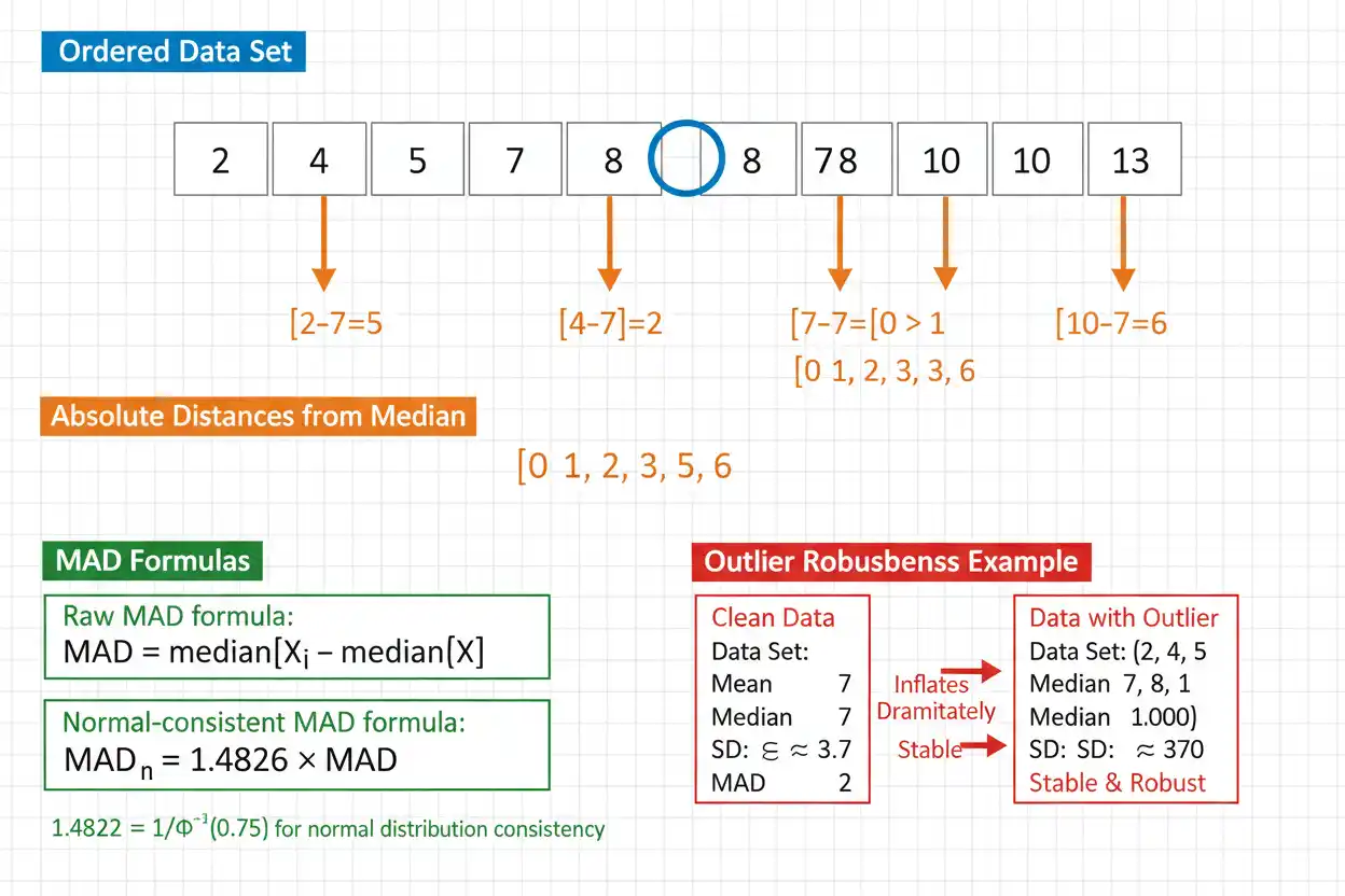
Median absolute deviation is a robust measure of statistical dispersion that describes the typical absolute distance of observations from the median rather than measuring spread through squared deviations from the arithmetic mean. For observations x₁, x₂, …, xₙ, the raw median absolute deviation is calculated by first finding the sample median, computing |xᵢ − median(x)| for every observation, and then taking the median of those absolute deviations. Because both the center and the spread calculation rely on medians, isolated extreme observations usually have much less influence on median absolute deviation than they have on variance or standard deviation, which makes MAD particularly useful for skewed data, contaminated samples, heavy-tailed distributions, and robust outlier analysis. A scaled version, commonly obtained by multiplying raw MAD by approximately 1.4826, is often used when a spread estimate comparable to the standard deviation of a normal distribution is desired. Raw MAD and scaled MAD are not interchangeable, however, so the convention should always be identified when formulas, thresholds, or software outputs are compared.
Median absolute deviation belongs to the broader toolkit of descriptive statistics within Statistics & Probability. It is built directly around the median, which gives the method much of its resistance to unusually large or small observations and distinguishes it from mean-centered measures of variability.
What Is Median Absolute Deviation?
Median absolute deviation measures the median distance of observations from their median.
For observations:
x₁, x₂, …, xₙ
first calculate:
m = Median(x)
Then calculate absolute deviations:
dᵢ = |xᵢ − m|
Finally:
MAD = Median(dᵢ)
or equivalently:
MAD = Median(|xᵢ − Median(x)|)
The result has the same measurement units as the original data.
If the observations are measured in kilograms, MAD is measured in kilograms.
If the observations are measured in seconds, MAD is measured in seconds.
Median Absolute Deviation Formula
The basic formula is:
MAD = Median(|xᵢ − m|)
where:
m = Median(x₁, x₂, …, xₙ)
Therefore:
MAD = Median(|xᵢ − Median(x)|)
The word absolute is important because distances below and above the center must not cancel one another.
For example:
|−5| = 5
and:
|5| = 5.
Both observations are equally distant from the median.
Simple Median Absolute Deviation Example
Consider:
1, 2, 3, 4, 5
The median is:
Calculate absolute deviations:
|1 − 3| = 2
|2 − 3| = 1
|3 − 3| = 0
|4 − 3| = 1
|5 − 3| = 2
The deviation values are:
2, 1, 0, 1, 2.
Sort them:
0, 1, 1, 2, 2.
Their median is:
Therefore:
MAD = 1
Why Absolute Deviations Are Used
Ordinary signed deviations from a central location can cancel.
For:
1, 2, 3, 4, 5
around median:
3
the deviations are:
−2, −1, 0, 1, 2.
Their sum is:
A zero sum clearly does not mean the observations have no spread.
Taking absolute values transforms the distances into:
2, 1, 0, 1, 2
so each departure contributes positively to the spread calculation.
The median then summarizes the typical absolute distance robustly.
Step-by-Step Calculation
To calculate median absolute deviation manually, use the following sequence.
First, sort the observations if necessary and find their median:
m = Median(x)
Next, calculate an absolute deviation for every observation:
|xᵢ − m|
Then sort those deviations.
Finally, calculate their median.
That final value is the raw MAD.
The method therefore involves two median calculations: one for the original observations and another for their absolute deviations.
Example With an Odd Sample Size
Consider:
4, 7, 9, 10, 15, 18, 22
The sample contains:
n = 7
observations.
The middle value is:
Median = 10.
Now calculate absolute deviations:
|4 − 10| = 6
|7 − 10| = 3
|9 − 10| = 1
|10 − 10| = 0
|15 − 10| = 5
|18 − 10| = 8
|22 − 10| = 12
Sort:
0, 1, 3, 5, 6, 8, 12
The central deviation is:
5
so:
MAD = 5.
Example With an Even Sample Size
Consider:
2, 4, 6, 10, 12, 18
There are:
n = 6
observations.
The two central observations are:
6 and 10.
Therefore:
Median = (6 + 10)/2
= 8.
Absolute deviations are:
|2 − 8| = 6
|4 − 8| = 4
|6 − 8| = 2
|10 − 8| = 2
|12 − 8| = 4
|18 − 8| = 10
Sort:
2, 2, 4, 4, 6, 10.
The two middle deviations are:
4 and 4.
Therefore:
MAD = 4.
Median Absolute Deviation Measures Spread, Not Center
The median and MAD describe different aspects of the data.
The median identifies:
central location.
MAD identifies:
typical absolute distance from that location.
For example, two data sets can both have:
Median = 50
while one has:
MAD = 2
and the other:
MAD = 25.
Their centers are identical, but the second distribution is much more dispersed around that center.
A useful robust summary can therefore report both:
Median ± MAD
while recognizing that this notation is descriptive rather than automatically a confidence interval.
Why MAD Is Called Robust
A robust statistic is relatively insensitive to a limited number of extreme observations or contaminated values.
Consider:
1, 2, 3, 4, 5
We already found:
Median = 3
MAD = 1.
Now replace the largest value 5 with:
1,000,000.
The data become:
1, 2, 3, 4, 1,000,000.
Median remains:
Absolute deviations are:
2, 1, 0, 1, 999,997.
Sorted:
0, 1, 1, 2, 999,997.
Therefore:
MAD = 1.
Despite an enormous change to the largest observation, MAD remains unchanged.
Compare With Standard Deviation
The standard deviation reacts strongly to extreme observations because squared deviations give large values disproportionate influence.
MAD uses:
absolute distance
and then takes:
a median
rather than averaging all distances.
Consequently, the observation:
1,000,000
can dramatically increase standard deviation while having no effect on raw MAD in the previous example.
This does not make standard deviation defective.
It means the two measures answer different questions and have very different robustness properties.
Breakdown Point
The median and median absolute deviation have high resistance to contamination.
Informally, nearly half of a sufficiently large sample can be contaminated before a median-based statistic can be driven arbitrarily far.
This contrasts sharply with mean-based quantities such as the arithmetic mean and standard deviation, where one sufficiently extreme observation can cause an arbitrarily large change.
That high breakdown resistance makes MAD attractive in applications where occasional gross errors or naturally extreme values are plausible.
Robustness does not mean the statistic can withstand unlimited contamination.
Raw MAD vs Scaled MAD
Two different quantities are often called “MAD.”
The raw median absolute deviation is:
MAD_raw = Median(|xᵢ − Median(x)|)
A scaled version is:
MAD_scaled = c × MAD_raw
where c is chosen for a particular reference distribution.
For normal-distribution consistency:
c ≈ 1.4826.
Therefore:
MAD_normal ≈ 1.4826 × MAD_raw.
The scaled form estimates a standard-deviation-like quantity under normality.
The raw form remains the direct median absolute distance.
Why the Normal Scaling Constant Is About 1.4826
For a standard normal random variable Z:
Median(|Z|) ≈ 0.67449.
Therefore, if a normal population has standard deviation σ:
Population raw MAD ≈ 0.67449σ.
To make MAD comparable to σ under normality, multiply by:
1/0.67449
which is approximately:
1.4826.
Thus:
MAD_scaled ≈ 1.4826 MAD_raw.
This scaling does not make the data normal.
It simply calibrates the robust spread measure to equal σ in the normal-distribution model at the population level.
Scaling Example
Suppose:
MAD_raw = 4.
The normal-consistent scaled MAD is:
MAD_scaled = 1.4826(4)
= 5.9304.
Therefore:
MAD_scaled ≈ 5.93.
If the data plausibly come from a normal-type distribution, this value can be interpreted on approximately the same scale as the standard deviation.
If the distribution is strongly non-normal, the scaled MAD remains a robust statistic, but its equality with population standard deviation is no longer expected.
Do Not Mix Raw and Scaled MAD
Suppose one software package reports:
MAD = 4
while another reports:
MAD = 5.93
for the same observations.
They may both be correct.
One may report:
raw MAD
while the other automatically multiplies by:
1.4826.
Before comparing results, determine which convention is being used.
This is especially important when MAD appears in outlier thresholds or standardized scores.
MAD vs Mean Absolute Deviation
The abbreviation MAD can also be used for mean absolute deviation, which is a different statistic.
Mean absolute deviation can be calculated as:
Mean(|xᵢ − center|)
where the center may be the mean or another chosen value.
Median absolute deviation instead uses:
Median(|xᵢ − Median(x)|).
The two differ in both:
- the center;
- the aggregation method.
Because terminology varies, writing the full phrase “median absolute deviation” avoids ambiguity.
Mean Absolute Deviation Example
For:
1, 2, 3, 4, 5
around center:
3
the absolute deviations are:
2, 1, 0, 1, 2.
Their mean is:
(2 + 1 + 0 + 1 + 2)/5
= 6/5
= 1.2.
Their median is:
Therefore:
Mean absolute deviation = 1.2
while:
Median absolute deviation = 1.
The two statistics should not be used interchangeably.
MAD and Standard Deviation Under Normality
For a perfectly normal population:
raw MAD ≈ 0.67449σ.
Therefore:
σ ≈ 1.4826 × raw MAD.
This makes scaled MAD useful as a robust estimate of standard deviation when a normal reference is appropriate.
For example, if:
raw MAD = 6.7449,
then:
scaled MAD ≈ 10.
A sample estimate will not generally equal this relationship exactly because of sampling variation.
The relationship describes the reference calibration.
MAD With an Extreme Upper Value
Consider:
10, 11, 12, 13, 14, 15, 1000.
Median:
Absolute deviations:
3, 2, 1, 0, 1, 2, 987.
Sorted:
0, 1, 1, 2, 2, 3, 987.
Therefore:
MAD = 2.
The extreme observation creates a deviation of:
987
but because MAD uses the middle deviation rather than their arithmetic average, that extreme value does not dominate the result.
MAD With an Extreme Lower Value
Consider:
−1000, 10, 11, 12, 13, 14, 15.
Median:
Absolute deviations:
1012, 2, 1, 0, 1, 2, 3.
Sorted:
0, 1, 1, 2, 2, 3, 1012.
Therefore:
MAD = 2.
The direction of the extreme value does not matter because absolute deviations discard sign.
Thus, MAD measures magnitude of central deviation rather than directional asymmetry.
MAD Does Not Measure Skewness
Because the calculation uses:
|xᵢ − Median|
a value 10 units below the median and one 10 units above it both contribute:
MAD therefore does not indicate whether dispersion occurs primarily to the left or right.
A strongly right-skewed and a strongly left-skewed distribution can have the same MAD.
Distributional direction must be examined with other statistics or graphical methods.
MAD measures robust spread, not asymmetry.
MAD and Kurtosis
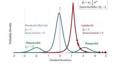
Kurtosis and median absolute deviation react very differently to extreme observations.
Kurtosis uses fourth-power deviations, which greatly magnify values far from the mean.
MAD uses median absolute distances, so isolated extreme values can have almost no influence on its result.
A sample can therefore have:
modest MAD
and:
extremely large kurtosis.
This combination can indicate that most observations are tightly concentrated while a small number lie very far into the tails.
MAD and Mode
The mode identifies the value or category occurring most frequently, whereas MAD measures numerical dispersion around the median.
Consider:
1, 1, 1, 5, 10, 20, 100.
The mode is:
The median is:
Absolute deviations from 5 are:
4, 4, 4, 0, 5, 15, 95.
The median of these is:
Therefore:
MAD = 4.
The mode and MAD answer entirely different descriptive questions.
MAD and Range
Range is:
Maximum − Minimum.
It depends completely on the two most extreme observations.
MAD depends on central ranks of absolute deviations.
For:
1, 2, 3, 4, 1000
the range is:
1000 − 1
= 999.
Median is:
Absolute deviations are:
2, 1, 0, 1, 997.
Therefore:
MAD = 1.
The contrast shows why range is highly sensitive to extremes while MAD is resistant.
MAD and Interquartile Range
Both MAD and IQR are robust measures of spread.
IQR is:
IQR = Q₃ − Q₁.
MAD is:
Median(|xᵢ − Median(x)|).
IQR describes the width of the central 50% of the original observations.
MAD describes the median absolute distance from the median.
They use different rank structures, so one cannot generally be converted into the other without distributional assumptions.
Both are useful when standard deviation is overly sensitive to extreme observations.
Normal-Distribution Relationship With IQR
For a normal distribution:
IQR ≈ 1.34898σ.
Therefore:
σ ≈ IQR/1.34898
≈ 0.7413 IQR.
Raw MAD satisfies:
MAD_raw ≈ 0.67449σ.
Thus, both IQR and MAD can be scaled to estimate σ under a normal reference model.
Neither relationship implies that robust scale measures are identical for arbitrary distributions.
Their different definitions cause them to respond differently to distribution shape.
MAD and Variance
Variance uses:
average squared deviation from the mean.
MAD uses:
median absolute deviation from the median.
Variance therefore gives every observation numerical influence and strongly weights large departures.
MAD gives much more influence to rank than to extreme magnitude.
For normal, uncontaminated data, variance-based estimators can be statistically more efficient.
For contaminated or heavy-tailed data, MAD can provide much greater stability.
The correct spread measure depends on the analytical objective.
Translation Invariance
Adding a constant to every observation does not change MAD.
Suppose:
yᵢ = xᵢ + c.
Then:
Median(y) = Median(x) + c.
Therefore:
|yᵢ − Median(y)|
becomes:
|xᵢ + c − Median(x) − c|
= |xᵢ − Median(x)|.
Thus:
MAD(Y) = MAD(X).
Moving the entire distribution left or right changes location but not dispersion.
Scaling Property
If every observation is multiplied by a constant a:
yᵢ = axᵢ,
then:
MAD(Y) = |a| MAD(X).
The absolute value is necessary because multiplying by a negative number reverses order but distances remain nonnegative.
For example, converting meters to centimeters multiplies every observation by:
Therefore, MAD is also multiplied by:
The spread changes numerically with the measurement scale in the same way as the original data.
Scale Example
Suppose distances in meters have:
MAD = 0.8 m.
Convert every observation to centimeters:
1 m = 100 cm.
Then:
MAD = 0.8(100)
= 80 cm.
The physical dispersion is unchanged.
Only the numerical unit changes.
This confirms that MAD has the same dimensional units as the underlying variable.
Negative Scaling Example
Suppose:
MAD(X) = 5.
Define:
Y = −3X.
Then:
MAD(Y) = |−3|(5)
= 15.
The sign reversal changes the direction of the scale but not absolute distance.
The factor of three stretches every distance threefold.
When MAD Equals Zero
MAD can equal zero even when not every observation is identical.
Consider:
1, 1, 1, 2, 100.
Median:
Absolute deviations:
0, 0, 0, 1, 99.
Their median is:
Therefore:
MAD = 0.
This occurs because at least half of the observations lie exactly at the median.
A zero MAD therefore does not necessarily imply zero overall variability.
Why Zero MAD Matters
A zero MAD can create difficulties for robust standardized scores because formulas divide by MAD.
Suppose:
MAD = 0.
Then an expression such as:
(xᵢ − Median)/MAD
is undefined.
This often occurs with:
- heavily discrete data;
- strongly repeated values;
- rounded measurements;
- small samples.
Alternative robust scale estimators or problem-specific methods may be necessary.
One should not replace zero with an arbitrary small number merely to make a formula work.
Modified Z-Score
A commonly used robust standardized score is:
Mᵢ = 0.6745(xᵢ − Median)/MAD_raw
where:
MAD_raw > 0.
The constant:
0.6745
approximately calibrates the score to ordinary z-scores under normality.
Because:
0.6745 ≈ 1/1.4826,
the same formula can also be understood using normal-scaled MAD.
Modified z-scores are useful for robust screening because the median and MAD are resistant to extreme observations.
Modified Z-Score Example
Consider:
10, 11, 12, 13, 14, 15, 100.
Median:
Raw MAD is:
For:
x = 100,
the modified z-score is:
M = 0.6745(100 − 13)/2
= 0.6745(87)/2
= 58.6815/2
≈ 29.34.
This is extremely large.
The observation is therefore far from the robust center relative to the robust spread.
Modified Z-Score Threshold
A frequently cited screening rule flags observations satisfying approximately:
|Mᵢ| > 3.5.
This is a heuristic, not a universal law.
An observation exceeding the threshold should be investigated rather than automatically deleted.
Formal outlier detection depends on the data-generating process, sample size, distribution, measurement system, and consequences of false positives.
A robust standardized score is evidence of unusualness, not proof of error.
Why Modified Z-Scores Can Outperform Ordinary Z-Scores With Outliers
Ordinary z-scores use:
zᵢ = (xᵢ − x̄)/s.
An extreme observation can increase both:
x̄
and:
s.
This can partially mask its own unusualness because the center and scale move toward it.
Modified z-scores use the median and MAD, which move much less under isolated contamination.
Therefore, the extreme observation often remains clearly separated from the central data.
This resistance is sometimes called reduced masking.
Masking
Masking occurs when extreme observations inflate a nonrobust scale estimate enough that they no longer appear as unusual as expected.
Suppose several large observations increase standard deviation substantially.
Their ordinary z-scores can become less extreme because:
denominator s
has increased.
MAD is much harder for a small number of extreme observations to inflate.
Therefore, robust screening can reveal potential anomalies that mean-and-standard-deviation methods partially conceal.
Swamping
Swamping is the opposite problem: ordinary observations may be incorrectly classified as unusual because contaminated center or scale estimates distort the reference distribution.
Robust statistics can reduce this effect when contamination is limited.
However, no outlier method completely eliminates false positives.
A flag should lead to investigation, not automatic exclusion.
The purpose of robust statistics is to reduce sensitivity, not to replace substantive judgment.
MAD and Margin of Error
A margin of error measures inferential uncertainty around an estimated parameter, whereas MAD is primarily a descriptive measure of observation-level spread.
A MAD of:
5 units
does not mean a population parameter has:
±5 units
of sampling uncertainty.
Likewise, multiplying raw MAD by 1.4826 produces a robust standard-deviation-like scale estimate under normality, not automatically a confidence margin.
Robust confidence procedures require an appropriate sampling-distribution or resampling method.
Spread and inferential precision should remain conceptually separate.
Median Absolute Deviation From Frequency Data
MAD can be calculated efficiently from a frequency table without expanding every repeated observation.
Suppose:
| Value | Frequency |
|---|---|
| 1 | 2 |
| 2 | 3 |
| 3 | 4 |
| 4 | 1 |
Total:
n = 10.
The median is determined from the:
5th and 6th
positions.
Positions 1–2 contain value 1.
Positions 3–5 contain value 2.
Positions 6–9 contain value 3.
Therefore:
Median = (2 + 3)/2
= 2.5.
Continue the Frequency Example
Calculate deviations from:
2.5.
For value 1:
|1 − 2.5| = 1.5
with frequency:
For value 2:
|2 − 2.5| = 0.5
with frequency:
For value 3:
|3 − 2.5| = 0.5
with frequency:
For value 4:
|4 − 2.5| = 1.5
with frequency:
Therefore, deviation frequencies are:
0.5 occurs 7 times
1.5 occurs 3 times.
The 5th and 6th deviations are both:
0.5.
Thus:
MAD = 0.5.
Why Frequency Weighting Works
A frequency table represents repeated observations compactly.
If value:
x = 10
has frequency:
50,
then its absolute deviation from the median occurs:
50 times.
The median of all deviations can therefore be located using cumulative frequency without listing those fifty values individually.
Frequency data preserve exact MAD calculation as long as the exact observed values and frequencies are available.
No approximation is necessary.
MAD From Grouped Data
If only grouped intervals are available, exact MAD usually cannot be recovered.
Suppose a class:
20–30
contains:
15 observations.
The table does not reveal exactly where those observations lie within the interval.
A rough approximation can replace each class by its midpoint and use frequencies as weights, but the result depends on that approximation.
Therefore, grouped-data MAD should be reported as estimated rather than exact when raw observations are unavailable.
Why Grouped MAD Can Be Inaccurate
MAD is based on ranked absolute distances from a median.
Grouping can obscure both:
- the exact median;
- the exact deviations around it.
A wide class containing the median is particularly problematic because many observations may have quite different distances from the true median while being represented by the same midpoint.
Narrower intervals retain more information.
Exact raw data are preferable whenever robust spread is an important analytical target.
MAD for Symmetric Data
Consider:
1, 2, 3, 4, 5, 6, 7.
Median:
Absolute deviations:
3, 2, 1, 0, 1, 2, 3.
Sorted:
0, 1, 1, 2, 2, 3, 3.
Therefore:
MAD = 2.
The distribution is symmetric around 4, and MAD provides a straightforward measure of its central absolute spread.
Symmetry is not required for the calculation.
MAD for Right-Skewed Data
Consider:
1, 2, 3, 4, 5, 7, 30.
Median:
Absolute deviations:
3, 2, 1, 0, 1, 3, 26.
Sorted:
0, 1, 1, 2, 3, 3, 26.
Therefore:
MAD = 2.
The distant upper-tail value contributes a deviation of 26 but does not change the median of the deviations.
This demonstrates the robustness of MAD under right skew and isolated upper extremes.
MAD for Left-Skewed Data
Consider:
−30, 1, 3, 4, 5, 6, 7.
Median:
Absolute deviations:
34, 3, 1, 0, 1, 2, 3.
Sorted:
0, 1, 1, 2, 3, 3, 34.
Therefore:
MAD = 2.
The statistic is again unaffected by the direction of the long tail.
This is why MAD must be combined with distributional shape measures when asymmetry matters.
MAD With Repeated Values
Repeated observations can make MAD very small or zero.
Consider:
5, 5, 5, 5, 6, 7, 100.
Median:
Absolute deviations:
0, 0, 0, 0, 1, 2, 95.
Median deviation:
Therefore:
MAD = 0.
The sample clearly has variability, but more than half of the observations equal the median.
The statistic accurately reflects the extremely concentrated central mass while ignoring the magnitude of the sparse upper tail.
Is Zero MAD a Failure?
No.
A zero value is a legitimate mathematical result.
It states that at least half of the absolute deviations occupy zero at the central deviation position.
What fails is any later procedure that assumes MAD must be positive.
For example, modified z-scores cannot divide by zero.
The solution is to choose a different scale estimator or modeling approach, not to alter the MAD artificially.
MAD and Sample Size
MAD can be calculated for small samples, but its values can be highly discrete because the statistic depends on one or two central ranked deviations.
With larger samples, it generally becomes a more stable estimator of a population MAD under suitable sampling conditions.
However, large sample size does not protect against:
- systematic sampling bias;
- inappropriate measurement;
- a badly defined population.
Robustness to extreme magnitudes is different from representativeness.
Sample MAD vs Population MAD
For a population random variable X with median m, population MAD can be defined as:
MAD_pop = Median(|X − m|).
A sample MAD estimates this population quantity.
Different random samples can produce different:
sample medians
and:
sample MADs.
Therefore, a sample MAD should not automatically be treated as the exact population spread.
Inference for population MAD requires accounting for sampling variability.
MAD and Normal Efficiency
MAD gains robustness at the cost of some statistical efficiency when the data are exactly normal and uncontaminated.
A standard deviation estimator can use more numerical information from every observation and is therefore more efficient under its ideal assumptions.
MAD intentionally sacrifices some of that sensitivity to obtain resistance against extreme contamination.
This is a common statistical tradeoff:
robustness versus model-specific efficiency.
The preferred measure depends on how credible the ideal model is.
MAD and Heavy-Tailed Data
Heavy-tailed data produce extreme observations more often than a normal distribution.
In such settings, standard deviation can fluctuate substantially between samples because squared deviations amplify tail events.
MAD remains driven by central ranks and can therefore provide a much more stable description of typical spread.
This does not mean tail behavior becomes unimportant.
It means MAD describes the central scale without allowing rare extremes to dominate it.
Separate tail measures can then be reported alongside it.
MAD and Log-Transformed Data
For positive multiplicative data, analysts sometimes transform:
Y = ln(X)
before calculating center and spread.
MAD on the log scale measures typical absolute log-distance from the log-scale median.
It is not generally equal to:
ln(MAD on the raw scale).
Nonlinear transformations change distances.
Therefore, a MAD calculated after logarithmic transformation should be interpreted on the transformed scale unless converted using a carefully defined multiplicative interpretation.
Linear Transformations
For:
Y = aX + b,
MAD follows:
MAD(Y) = |a|MAD(X).
The additive constant:
b
does not affect spread.
The multiplicative factor:
|a|
rescales every distance.
This simple transformation property makes MAD easy to interpret under ordinary unit conversions and affine changes.
MAD and Data Standardization
A robust standardized variable can be created using a scaled MAD:
z_robust = (x − Median)/MAD_scaled
when:
MAD_scaled > 0.
Because:
MAD_scaled ≈ 1.4826 MAD_raw
under normal calibration, this robust score resembles an ordinary z-score scale for approximately normal central data while remaining less sensitive to extreme observations.
The exact threshold used for decision-making should still be appropriate to the application.
Ordinary Z-Score vs Robust Z-Score
Ordinary:
z = (x − x̄)/s
uses a nonrobust center and spread.
Robust:
z_R = (x − Median)/MAD_scaled
uses resistant alternatives.
If data contain no significant contamination and follow a well-behaved symmetric distribution, both scores may tell a similar story.
If a few extremes are present, ordinary mean and standard deviation can shift considerably while median and MAD remain much more stable.
That difference is precisely why robust standardized scores exist.
MAD Is Not a Probability
Suppose:
MAD = 5.
This does not mean:
50% of values are within exactly ±5
under every finite-sample convention, nor does it mean:
P(|X − Median| ≤ 5) = 0.5
in every discrete or tied setting.
The population interpretation is quantile-based, but repeated values can create probability masses at the MAD boundary.
In continuous distributions without ties, the central interpretation is cleaner.
MAD should be treated as a scale quantile, not a probability statement by itself.
MAD and the Central 50%
Because MAD is the median of absolute deviations, it identifies the 50th percentile of the distance-from-median distribution.
This differs from IQR, which spans from the 25th to the 75th percentile of the original data.
Both involve central 50% concepts, but on different variables:
IQR → original observations
MAD → absolute deviations from median.
Therefore, they should not be interpreted as equivalent numerical widths.
Comparing Groups With MAD
Suppose:
Group A: Median = 50, MAD = 3
Group B: Median = 50, MAD = 12.
Both groups have the same central location.
Group B has much greater robust dispersion around that center.
This comparison is especially informative when extreme observations would make standard deviations unstable.
However, if measurement scales differ substantially between groups, absolute MAD values may not be directly comparable without additional context.
Relative MAD
A relative robust spread can sometimes be constructed by comparing MAD with a meaningful positive median:
Relative MAD = MAD/Median
or:
Relative MAD% = (MAD/Median) × 100%.
This is not as universally standardized as the coefficient of variation, and interpretation becomes problematic when the median is:
zero,
near zero,
or negative.
It should therefore be used only when the ratio scale and denominator have a meaningful interpretation.
Missing Values
Missing observations should be excluded or handled according to a clearly defined missing-data method before calculating MAD.
Coding missing values as:
0
can change both the median and the absolute deviations.
Suppose valid data are:
10, 20, 30.
Median:
If two missing values are incorrectly coded as zero:
0, 0, 10, 20, 30
the median becomes:
The resulting MAD describes the corrupted data rather than the valid observations.
Measurement Resolution
Low-resolution measurements can produce many ties.
Suppose a sensor rounds every value to the nearest:
10 units.
A large proportion of readings can become identical.
MAD can then become:
0
even though underlying continuous variation exists.
This is not an arithmetic error.
It reflects the information resolution of the observed data.
A more precise instrument or a different robust scale estimator may be needed if finer variability must be measured.
Common Median Absolute Deviation Mistakes
A common mistake is calculating deviations from the arithmetic mean instead of from the median. The standard median absolute deviation is centered on the median.
Another error is averaging the absolute deviations instead of taking their median, which produces a mean absolute deviation rather than MAD.
Analysts also frequently compare a raw MAD with a scaled MAD without noticing the approximately 1.4826 factor.
Another mistake is using:
1.4826
as though it were universally required. It is specifically a normal-consistency scaling convention.
Using modified z-scores when:
MAD = 0
creates division by zero and requires another approach.
Potential outliers identified with robust thresholds should not be automatically deleted.
Finally, MAD should not be interpreted as a confidence interval, standard error, or directional measure of skewness.
How to Calculate Median Absolute Deviation Step by Step
Begin with the valid numerical observations.
Find the sample median:
m = Median(x).
For every observation, calculate:
dᵢ = |xᵢ − m|.
Sort the absolute deviations.
Calculate:
Median(d).
The result is:
MAD_raw.
If a normal-consistent scale estimate is specifically required, calculate:
MAD_scaled ≈ 1.4826 × MAD_raw.
Always state whether the reported result is raw or scaled.
Full Worked Example
Consider:
3, 5, 7, 8, 9, 12, 20, 25, 100
There are:
n = 9
observations.
Step 1: Find the Median
The fifth observation is:
Therefore:
Median = 9.
Step 2: Calculate Absolute Deviations
|3 − 9| = 6
|5 − 9| = 4
|7 − 9| = 2
|8 − 9| = 1
|9 − 9| = 0
|12 − 9| = 3
|20 − 9| = 11
|25 − 9| = 16
|100 − 9| = 91
Step 3: Sort the Deviations
0, 1, 2, 3, 4, 6, 11, 16, 91
Step 4: Find Their Median
The fifth deviation is:
Therefore:
MAD_raw = 4.
Calculate the Scaled MAD
Using normal consistency:
MAD_scaled ≈ 1.4826(4)
= 5.9304.
Therefore:
MAD_scaled ≈ 5.93.
The raw MAD tells us that the median absolute distance from the sample median is four units.
The scaled version translates that robust spread onto a standard-deviation-like scale under the normal reference convention.
Outlier Screening in the Worked Example
For:
x = 100
use:
Median = 9
and:
MAD_raw = 4.
Modified z-score:
M = 0.6745(100 − 9)/4
= 0.6745(91)/4
= 61.3795/4
≈ 15.34.
This is far beyond the commonly used screening magnitude:
3.5.
Therefore, 100 would be strongly flagged for investigation under this robust rule.
The statistical flag does not prove the value is invalid.
Compare an Ordinary Observation
For:
x = 12
the modified z-score is:
M = 0.6745(12 − 9)/4
= 0.6745(3)/4
= 2.0235/4
≈ 0.506.
This value lies close to the robust center.
Thus, the same MAD scale distinguishes an ordinary observation from the extreme upper value without allowing the extreme value to inflate the scale substantially.
Full Zero-MAD Example
Consider:
5, 5, 5, 5, 6, 20, 100.
Median:
Absolute deviations:
0, 0, 0, 0, 1, 15, 95.
Sorted deviations are already:
0, 0, 0, 0, 1, 15, 95.
The central deviation is:
Therefore:
MAD = 0.
The data still vary substantially.
The result simply reflects that more than half of the sample is concentrated exactly at the median.
What to Do When MAD Is Zero
If the goal is merely descriptive reporting, a zero MAD can be reported directly along with other measures showing the remaining dispersion.
If robust standardization or outlier detection is required, consider a method that remains defined for highly tied data, depending on the problem.
Possible alternatives may include:
- IQR-based rules;
- other robust scale estimators;
- discrete-data models;
- domain-specific thresholds.
The correct solution depends on why the data contain so many repeated values.
There is no universal replacement formula.
How to Report MAD
A clear report identifies both the center and spread convention.
For example:
“The sample median was 9 units and the raw median absolute deviation was 4 units.”
If normal scaling is used:
“The raw MAD was 4 units, corresponding to a normal-consistent scaled MAD of approximately 5.93 units.”
This wording prevents ambiguity.
When a robust outlier procedure is used, also state the rule or threshold rather than assuming every reader uses the same convention.
When to Use Median Absolute Deviation
MAD is particularly useful when:
- the distribution is skewed;
- extreme observations are present;
- measurement contamination is possible;
- a robust scale estimate is required;
- median is a more appropriate center than mean;
- robust anomaly screening is needed.
It is also useful for exploratory analysis because comparing MAD with standard deviation can reveal whether extreme values are exerting substantial influence on conventional spread estimates.
MAD is especially informative when used alongside a distribution graph rather than as an isolated number.
When Standard Deviation May Be Preferable
Standard deviation may be preferable when:
- the arithmetic mean is the target center;
- squared-error methods are substantively appropriate;
- the population is well modeled by a light-tailed distribution;
- efficiency under a normal model is important;
- variance-based inferential procedures are being used.
MAD is not intended to replace standard deviation in every analysis.
The two measures embody different assumptions and priorities.
A robust method becomes valuable when resistance to contamination matters more than maximum efficiency under an ideal model.
Frequently Asked Questions About Median Absolute Deviation
What is median absolute deviation?
It is the median of the absolute distances between observations and their median.
What is the formula?
MAD = Median(|xᵢ − Median(x)|)
What does MAD measure?
It measures robust dispersion around the median.
Does MAD have the same units as the data?
Yes.
Is MAD a measure of center?
No. It is a measure of spread.
What measure of center is used?
The median.
Why are absolute values used?
They prevent negative and positive deviations from canceling.
Why is the median used twice?
The first median locates the center, and the second median robustly summarizes the absolute deviations from that center.
Is MAD robust to outliers?
Yes, comparatively.
Can one extreme value leave MAD unchanged?
Yes.
Why?
Because the median of the deviations depends mainly on their central ranks rather than the largest magnitude.
Is MAD the same as mean absolute deviation?
No.
What is mean absolute deviation?
It averages absolute deviations instead of taking their median.
What is raw MAD?
Median(|xᵢ − Median(x)|)
without a scaling factor.
What is scaled MAD?
A raw MAD multiplied by a chosen consistency factor.
What normal-consistency factor is commonly used?
Approximately:
1.4826.
Why 1.4826?
Because a normal population has:
raw MAD ≈ 0.67449σ
and:
1/0.67449 ≈ 1.4826.
Does multiplying by 1.4826 make the data normal?
No.
What does it do?
It calibrates MAD so that its population value matches σ under a normal reference distribution.
Should every MAD be multiplied by 1.4826?
No.
Why not?
Raw and scaled MAD serve different reporting conventions, and the factor is specifically tied to normal consistency.
Can MAD be zero?
Yes.
Does MAD = 0 mean all observations are identical?
No.
When can MAD equal zero?
When at least enough observations are concentrated at the median that the median absolute deviation is zero.
Can modified z-scores be calculated when MAD = 0?
Not with the ordinary formula because it would require division by zero.
What is the modified z-score formula?
A common form is:
Mᵢ = 0.6745(xᵢ − Median)/MAD_raw
What threshold is commonly used?
A frequently used screening rule is:
|Mᵢ| > 3.5.
Does crossing 3.5 prove an observation is wrong?
No. It flags the observation for investigation.
Is MAD sensitive to whether an extreme value is above or below the median?
No. Absolute deviations remove direction.
Does MAD measure skewness?
No.
Can a right-skewed and left-skewed sample have the same MAD?
Yes.
Can MAD be calculated for negative values?
Yes.
Can MAD be calculated for decimal values?
Yes.
Can MAD be calculated from a frequency table?
Yes, exactly when exact values and their frequencies are available.
Can MAD be calculated exactly from grouped intervals?
Usually not if the raw observations are unavailable.
Why not?
Grouping hides exact locations of observations and therefore exact distances from the median.
Is grouped MAD an approximation?
Usually yes when class midpoints are substituted for raw values.
What happens if all observations increase by 10?
MAD remains unchanged.
What happens if all observations are multiplied by 5?
MAD is multiplied by 5.
What happens if observations are multiplied by −5?
MAD is multiplied by:
|−5| = 5.
Is MAD affected by changing measurement units?
Its numerical value changes by the same scale conversion as the data.
Is MAD the same as IQR?
No.
How are they different?
IQR measures the distance between Q₁ and Q₃, while MAD measures the median absolute distance from the median.
Is MAD the same as range?
No. Range depends on minimum and maximum and is highly sensitive to extremes.
Is MAD the same as standard deviation?
No.
Which is more resistant to extreme observations?
MAD.
Is standard deviation ever better?
Yes. Under suitable light-tailed models such as normality, standard-deviation estimators can be more efficient and integrate naturally with many classical inferential procedures.
Can MAD be used as a standard-deviation estimate?
A scaled MAD can estimate σ robustly under a normal-reference model.
Is MAD a margin of error?
No.
Is MAD a standard error?
No.
Can MAD be used in robust standardized scores?
Yes.
Is MAD useful for outlier detection?
Yes, especially when mean and standard deviation could themselves be distorted by extreme observations.
Can two data sets have the same MAD but very different tails?
Yes.
Does MAD describe the entire distribution?
No. It is a one-number robust measure of spread.
What should be reported with MAD?
At minimum, the median and whether MAD is raw or scaled should be clear.
What is the biggest practical advantage of MAD?
It summarizes typical central spread while remaining resistant to a limited number of extreme observations.
What is its main limitation?
It can ignore substantial tail magnitude and can become zero in highly tied data, making some robust-standardization formulas undefined.
What is the most important rule when calculating median absolute deviation?
Find deviations from the median, take their absolute values, take the median of those deviations, and state explicitly whether the final result is the raw MAD or a scaled version such as the 1.4826 normal-consistent form.