
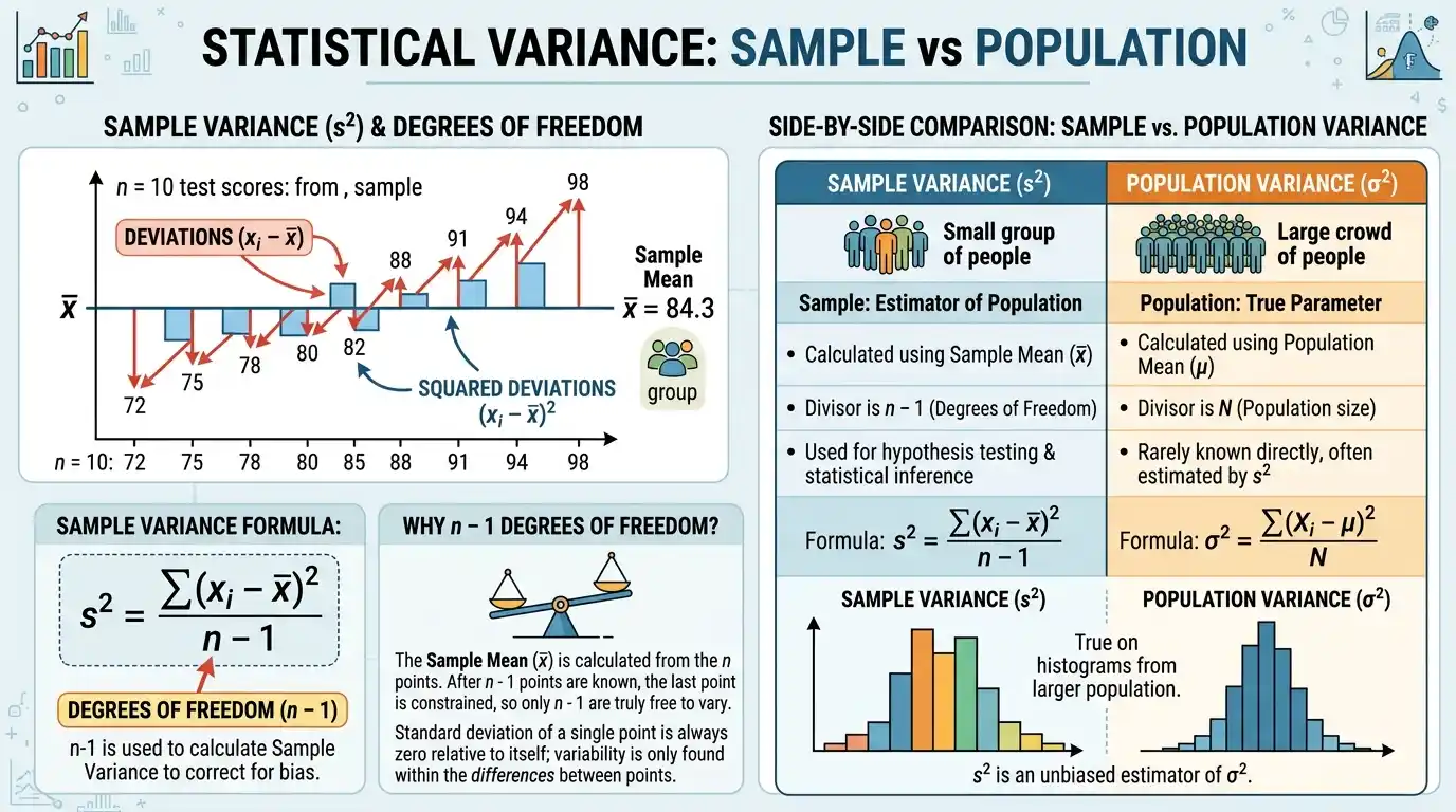

Sample variance is a measure of statistical dispersion that describes how widely observations in a sample are spread around their sample mean while, in its conventional form, using a denominator of n − 1 rather than n. For observations x₁, x₂, …, xₙ with sample mean x̄, the standard formula is s² = Σ(xᵢ − x̄)²/(n − 1), where the deviations are squared so positive and negative differences cannot cancel and observations farther from the center receive greater influence. The n − 1 denominator, commonly associated with Bessel’s correction, is especially important when the sample is being used to estimate the variance σ² of a larger population because the sample mean has already been estimated from the same observations. Under standard independent, identically distributed sampling with finite variance, this conventional sample variance is an unbiased estimator of population variance, meaning its expected value across repeated samples equals σ². Sample variance is therefore both a descriptive measure of observed spread and a fundamental inferential statistic that underlies sample standard deviation, standard errors, t procedures, regression, analysis of variance, and many other statistical methods.
Within descriptive statistics and the broader Statistics & Probability framework, sample variance should always be distinguished from population variance. The formulas look very similar, but the denominator and statistical interpretation differ because one describes a known population while the other is commonly used to estimate population variability from incomplete information.
What Is Sample Variance?
Sample variance measures average squared dispersion around the sample mean, with the conventional estimator dividing the squared-deviation total by:
n − 1
rather than:
n.
For a sample:
x₁, x₂, …, xₙ
first calculate:
x̄ = Σxᵢ/n
Then calculate every deviation:
xᵢ − x̄
Square those deviations:
(xᵢ − x̄)²
Add them and divide by:
n − 1.
The result is sample variance:
s².
Sample Variance Formula
The standard formula is:
s² = Σ(xᵢ − x̄)²/(n − 1)
where:
- s² = sample variance
- xᵢ = an individual sample observation
- x̄ = sample mean
- n = sample size
- Σ = sum over all sample observations
This formula is ordinarily used when the sample represents observations drawn from a broader population and the objective is to estimate that population’s variance.
Sample Mean Formula
Before calculating sample variance, find:
x̄ = Σxᵢ/n
Suppose the sample is:
2, 4, 6, 8
Then:
x̄ = (2 + 4 + 6 + 8)/4
= 20/4
= 5
The sample mean becomes the reference point for every squared deviation.
Simple Sample Variance Example
Consider:
2, 4, 6, 8
We already found:
x̄ = 5.
Deviations are:
−3, −1, 1, 3
Squared deviations are:
9, 1, 1, 9
Their sum is:
Sample size:
n = 4
so:
n − 1 = 3.
Therefore:
s² = 20/3
≈ 6.667
The sample variance is approximately:
6.67 square units.
Why Sample Variance Uses Squared Deviations
If ordinary deviations were added, they would cancel.
For the sample:
2, 4, 6, 8
with mean 5:
−3 − 1 + 1 + 3 = 0.
A zero result clearly does not mean there is no variability.
Squaring gives:
9 + 1 + 1 + 9 = 20
so every deviation contributes positively.
Squaring also emphasizes observations farther from the mean, which gives variance important mathematical properties while making it sensitive to extreme observations.
Why Divide by n − 1?
The denominator n − 1 is connected to the fact that the sample mean is estimated from the same observations whose variability is being measured.
Once:
x̄
has been calculated, the sample deviations satisfy:
Σ(xᵢ − x̄) = 0.
Therefore, if:
n − 1
of the deviations are known, the final deviation is already determined.
Only:
n − 1
deviations are free to vary independently.
This is the origin of the one-degree-of-freedom loss.
Degrees of Freedom
For the ordinary sample variance:
df = n − 1.
Suppose:
n = 10.
Then:
df = 9.
If the first nine deviations from x̄ are known, the tenth must take exactly the value needed to make their total zero.
Therefore, the data contain only nine independent pieces of deviation information after the sample mean has been estimated.
Bessel’s Correction
Using:
n − 1
instead of n is commonly called Bessel’s correction.
The reason is statistical rather than arbitrary.
If a random sample is drawn independently from a population with finite variance σ², then the conventional estimator satisfies:
E(s²) = σ².
Thus, sample variance using n − 1 is unbiased for population variance under the standard sampling framework.
If the squared deviations were divided by n instead, the resulting estimator would be biased downward on average.
Why Dividing by n Underestimates Population Variance
The sample mean:
x̄
is chosen from the sample itself.
It is the value that minimizes:
Σ(xᵢ − c)²
over all constants c.
Therefore, squared deviations around x̄ tend to be smaller than squared deviations around the unknown population mean μ.
If that artificially reduced squared-deviation total were simply divided by n, the resulting statistic would systematically underestimate σ².
The n − 1 correction compensates exactly for that expected downward bias under the usual assumptions.
Sample Variance vs Population Variance
Population variance is:
σ² = Σ(xᵢ − μ)²/N.
Sample variance is conventionally:
s² = Σ(xᵢ − x̄)²/(n − 1).
The key distinctions are:
Population → μ and N
Sample → x̄ and n − 1
Suppose:
2, 4, 6, 8
are the complete population.
Then:
σ² = 20/4
= 5.
If they are instead a sample used to estimate a larger population variance:
s² = 20/3
≈ 6.667.
The observations are identical, but the statistical objectives differ.
When Should You Divide by n?
Dividing by n is appropriate when the values constitute the entire finite population being described:
σ² = Σ(xᵢ − μ)²/N.
It may also appear in maximum-likelihood or empirical-moment formulations under particular modeling conventions.
However, when “sample variance” refers to the standard unbiased estimator of an unknown population variance, the conventional denominator is:
n − 1.
Always identify the purpose of the calculation rather than choosing a denominator mechanically.
Sample Variance Step by Step
To calculate sample variance manually, first calculate:
x̄ = Σxᵢ/n.
Next subtract x̄ from every observation.
Square each deviation.
Add all squared deviations.
Then divide by:
n − 1.
The result is:
s².
If the sample standard deviation is required, take the square root:
s = √s².
Worked Example With Five Observations
Consider:
3, 5, 7, 9, 11
Sample mean:
x̄ = 35/5
= 7.
Deviations:
−4, −2, 0, 2, 4.
Squared deviations:
16, 4, 0, 4, 16.
Sum:
Because:
n = 5,
we have:
n − 1 = 4.
Therefore:
s² = 40/4
= 10.
The sample variance is:
Sample Standard Deviation
Sample standard deviation is:
s = √s².
For:
s² = 10
we obtain:
s = √10
≈ 3.162.
Thus:
Sample variance = 10 square units
while:
Sample standard deviation ≈ 3.16 original units.
Standard deviation is often easier to interpret because it returns to the original measurement scale.
Why Sample Variance Has Squared Units
Suppose observations are measured in:
kilograms.
Each deviation:
xᵢ − x̄
is measured in kilograms.
Squaring gives:
kilograms².
Averaging the squared deviations with the n − 1 denominator leaves those squared units unchanged.
Therefore:
Sample variance is measured in kg².
The corresponding sample standard deviation is measured in kilograms.
Sample Variance Cannot Be Negative
Every term:
(xᵢ − x̄)²
is nonnegative.
Therefore:
Σ(xᵢ − x̄)² ≥ 0.
Since:
n − 1 > 0
for n > 1:
s² ≥ 0.
A correctly calculated sample variance cannot be negative.
A negative result indicates a calculation or numerical precision problem.
When Sample Variance Equals Zero
If every sample observation is identical:
8, 8, 8, 8
then:
x̄ = 8.
Every deviation is:
Therefore:
s² = 0.
Conversely, if at least two sample observations differ, the squared-deviation sum is positive and the sample variance must exceed zero.
Can Sample Variance Be Calculated for n = 1?
For the conventional estimator:
s² = Σ(xᵢ − x̄)²/(n − 1),
a sample with:
n = 1
would require division by:
Therefore, conventional sample variance is undefined for a one-observation sample.
At least:
n = 2
observations are required.
This reflects the fact that one observation provides no independent information about variation around an estimated mean.
Sample Variance With Two Observations
Suppose:
4, 10.
Sample mean:
x̄ = 7.
Deviations:
−3, 3.
Squared deviations:
9, 9.
Total:
Because:
n − 1 = 1,
sample variance is:
s² = 18.
Sample standard deviation is:
√18 ≈ 4.243.
With only two observations, the variance can be calculated but remains a highly uncertain estimator of population variability.
Computational Sample Variance Formula
An equivalent shortcut formula is:
s² = [Σxᵢ² − (Σxᵢ)²/n]/(n − 1)
Another equivalent form is:
s² = [Σxᵢ² − nx̄²]/(n − 1).
These identities avoid calculating each deviation individually when:
Σx
and:
Σx²
are already available.
They are mathematically equivalent to the ordinary deviation formula.
Deriving the Shortcut Formula
Start with:
Σ(xᵢ − x̄)²
Expand:
Σ[xᵢ² − 2x̄xᵢ + x̄²]
which gives:
Σxᵢ² − 2x̄Σxᵢ + nx̄².
Since:
Σxᵢ = nx̄,
we obtain:
Σxᵢ² − 2nx̄² + nx̄²
= Σxᵢ² − nx̄².
Because:
nx̄² = (Σxᵢ)²/n,
the alternative identity follows immediately.
Shortcut Formula Example
For:
2, 4, 6, 8
calculate:
Σx = 20
and:
Σx² = 4 + 16 + 36 + 64
= 120.
Then:
s² = [120 − 20²/4]/3
= [120 − 400/4]/3
= (120 − 100)/3
= 20/3
≈ 6.667.
The result matches the direct squared-deviation calculation.
Numerical Stability
Although the shortcut identity is exact mathematically, naïve computer implementations can lose numerical precision when observations are extremely large while their actual spread is small.
For example, values close to:
1,000,000,000
produce enormous:
Σx²
and:
(Σx)²/n
terms.
Their difference may be relatively tiny.
Subtracting nearly equal large floating-point numbers can create cancellation error.
Reliable statistical implementations therefore often use numerically stable variance algorithms.
Sample Variance From a Frequency Table
When exact values are summarized by frequency:
fᵢ,
the sample mean is:
x̄ = Σfᵢxᵢ/n
where:
n = Σfᵢ.
Sample variance is:
s² = Σfᵢ(xᵢ − x̄)²/(n − 1).
This gives exactly the same result as expanding every repeated observation individually.
Frequency notation simply makes the calculation more efficient.
Frequency-Table Example
Suppose:
| Value | Frequency |
|---|---|
| 1 | 2 |
| 2 | 3 |
| 4 | 1 |
Total sample size:
n = 6.
Mean:
x̄ = [1(2) + 2(3) + 4(1)]/6
= 12/6
= 2.
Weighted squared deviations are:
2(1 − 2)² = 2
3(2 − 2)² = 0
1(4 − 2)² = 4.
Total:
Therefore:
s² = 6/(6 − 1)
= 6/5
= 1.2.
Sample Variance From Relative Frequencies
A relative frequency is:
rᵢ = fᵢ/n.
Because:
fᵢ = nrᵢ,
the sample squared-deviation total can be written:
Σfᵢ(xᵢ − x̄)² = nΣrᵢ(xᵢ − x̄)².
Therefore:
s² = [n/(n − 1)]Σrᵢ(xᵢ − x̄)².
This formula shows why relative frequencies alone may not be sufficient to recover conventional sample variance unless:
n
is also known.
The n/(n − 1) correction depends explicitly on sample size.
Relative-Frequency Example
Suppose:
| Value | Relative Frequency |
|---|---|
| 1 | 2/6 |
| 2 | 3/6 |
| 4 | 1/6 |
and:
n = 6.
Mean:
x̄ = 2.
The relative-frequency weighted squared deviation is:
(2/6)(1 − 2)² + (3/6)(2 − 2)² + (1/6)(4 − 2)²
= 2/6 + 0 + 4/6
= 1.
Then:
s² = 6/5
= 1.2.
This matches the frequency-count calculation.
Sample Variance From Grouped Data
When only class intervals are available, sample variance can be approximated with class midpoints.
Let:
mᵢ = midpoint of class i
and:
fᵢ = class frequency.
Approximate sample mean:
x̄ ≈ Σfᵢmᵢ/n.
Approximate sample variance:
s² ≈ Σfᵢ(mᵢ − x̄)²/(n − 1).
The result is approximate because every observation within a class is represented by the same midpoint.
Grouped Sample Variance Example
Suppose:
| Interval | Frequency | Midpoint |
|---|---|---|
| 0–10 | 4 | 5 |
| 10–20 | 6 | 15 |
| 20–30 | 10 | 25 |
Total:
n = 20.
Approximate mean:
x̄ ≈ [4(5) + 6(15) + 10(25)]/20
= 360/20
= 18.
Weighted squared-deviation total:
4(5 − 18)² + 6(15 − 18)² + 10(25 − 18)²
= 676 + 54 + 490
= 1220.
Therefore:
s² ≈ 1220/19
≈ 64.21.
Why Grouped Sample Variance Is Approximate
The midpoint method replaces every observation in an interval with one representative value.
For a:
20–30
class, values such as:
20.1
and:
29.9
are both replaced by:
Because sample variance depends on squared distances, this loss of within-class information can materially affect the result.
Narrower classes generally reduce the approximation error.
Raw observations should be used when exact variance is required.
Sample Variance and Outliers
Sample variance is highly sensitive to extreme observations.
Suppose:
1, 2, 3, 4, 5
The sample mean is:
Squared-deviation total:
Therefore:
s² = 10/4
= 2.5.
Now replace 5 with:
The data become:
1, 2, 3, 4, 100.
One changed observation will cause the variance to increase dramatically.
Calculate the Extreme-Value Example
For:
1, 2, 3, 4, 100
sample mean:
x̄ = 110/5
= 22.
Deviations:
−21, −20, −19, −18, 78.
Squared deviations:
441, 400, 361, 324, 6084.
Sum:
Therefore:
s² = 7610/4
= 1902.5.
The sample variance increased from:
2.5
to:
1902.5.
This demonstrates why outlier detection can be important when interpreting variance-based summaries.
Why Outliers Have So Much Influence
If one observation lies:
2 units
from the mean, its squared contribution is:
An observation:
20 units
from the mean contributes:
The second distance is ten times larger but contributes one hundred times as much.
Sample variance therefore treats extreme deviations as especially important rather than as small perturbations.
This is useful in squared-error modeling but can make the statistic unstable in heavy-tailed or contaminated data.
Sample Variance vs Median Absolute Deviation
Median absolute deviation is a robust measure based on typical absolute distance from the median.
Sample variance instead uses:
squared distance from the sample mean.
For contaminated data, the two can differ enormously.
Variance deliberately represents extreme squared deviations strongly, whereas MAD resists them.
Neither statistic is universally preferable.
The appropriate measure depends on whether the analysis should emphasize total squared dispersion or robust central spread.
Sample Variance vs Range
The range is:
Maximum − Minimum.
It uses only two observations.
Sample variance uses every observation.
Consider:
A = 0, 5, 5, 5, 10
and:
B = 0, 0, 5, 10, 10.
Both have:
Range = 10.
Their sample variances differ because their internal distributions differ.
Variance therefore contains substantially more information about overall dispersion than endpoint span alone.
Sample Variance and Skewness
Skewness describes directional asymmetry, whereas sample variance measures squared dispersion without direction.
A deviation:
−10
and a deviation:
+10
both contribute:
100
to the variance numerator.
Therefore, variance cannot reveal whether extreme values occur primarily above or below the center.
A sample can have high variance and zero skewness, or low variance and substantial skewness on a narrow numerical scale.
The measures describe different properties.
Sample Variance and Standard Error
A standard error measures the sampling variability of an estimator, while sample variance measures variability among the observations themselves.
For the sample mean, a common estimated standard error is:
SE(x̄) = s/√n
under the usual independent sampling assumptions.
Because:
s = √s²,
sample variance contributes directly to the standard-error calculation.
However:
sample variance ≠ standard error.
One describes observation-level dispersion; the other describes estimator uncertainty.
Example Connecting Variance and Standard Error
Suppose:
s² = 100
so:
s = 10.
If:
n = 25,
then:
SE(x̄) = 10/√25
= 10/5
= 2.
Therefore:
Sample variance = 100
Sample standard deviation = 10
Estimated standard error of mean = 2.
These three quantities are related but measure different statistical concepts.
Sample Variance and Sample Size
Increasing sample size does not automatically make the sample variance smaller.
A larger sample can contain more extreme observations and may estimate a population with substantial variability.
What larger n generally does under suitable sampling is make:
s²
a more stable estimator of:
σ².
The spread of the underlying population remains what it is.
Sample size improves estimation precision rather than mechanically shrinking the population variability being estimated.
Expected Value of Sample Variance
Under independent identically distributed sampling with finite population variance σ²:
E(s²) = σ².
This is the formal unbiasedness property of the n − 1 estimator.
It does not mean:
s² = σ²
for every sample.
Individual samples can produce values above or below the true population variance.
Unbiasedness is a long-run expectation across repeated samples.
Unbiased Does Not Mean Exact
Suppose the true population variance is:
σ² = 25.
One random sample might produce:
s² = 18.
Another might produce:
s² = 31.
Another might produce:
s² = 24.
The estimator is unbiased if the average across all possible repeated samples equals 25 under the model.
No single sample is guaranteed to reproduce the population variance exactly.
This distinction between estimator expectation and realized estimate is fundamental.
Is Sample Standard Deviation Unbiased?
Although:
s²
is unbiased for σ² under standard assumptions,
s = √s²
is generally not an exactly unbiased estimator of σ.
The square-root transformation is nonlinear.
Therefore:
E(s) ≠ σ
in general.
The bias becomes small for sufficiently large samples under many common conditions, but the exact distinction matters statistically.
Unbiased variance does not imply unbiased standard deviation.
Maximum-Likelihood Variance Estimate
For independent normal observations with unknown μ and σ², the maximum-likelihood estimator of variance is:
σ̂²_ML = Σ(xᵢ − x̄)²/n.
This differs from the conventional unbiased sample variance:
s² = Σ(xᵢ − x̄)²/(n − 1).
The maximum-likelihood estimator uses:
n
because it optimizes the likelihood.
The unbiased estimator uses:
n − 1
to correct expected downward bias.
Both can be legitimate depending on the statistical objective.
Descriptive Variance With Denominator n
Sometimes an analyst wants only the average squared deviation of the observed sample values themselves, without using the statistic as an unbiased estimator of a larger population variance.
Then one may calculate:
m₂ = Σ(xᵢ − x̄)²/n.
This is the sample’s second central moment.
It should not be silently confused with the conventional:
s²
definition using n − 1.
Explicitly naming the convention prevents denominator disputes.
Sample Variance Under Translation
Suppose every observation has the same constant b added:
Y = X + b.
Then:
s²_Y = s²_X.
Adding a constant shifts both every observation and the sample mean by b.
Therefore:
yᵢ − ȳ = xᵢ − x̄.
The deviations remain unchanged.
Translation changes location but not sample variance.
Translation Example
Suppose:
X = 1, 3, 5.
Mean:
x̄ = 3.
Squared deviations:
4, 0, 4.
Sample variance:
s² = 8/2
= 4.
Add:
100
to every value:
Y = 101, 103, 105.
The new mean is:
103
and the deviations remain:
−2, 0, 2.
Therefore:
s²_Y = 4.
Sample Variance Under Scaling
If every observation is multiplied by a constant a:
Y = aX,
then:
s²_Y = a²s²_X.
Every deviation is multiplied by a:
yᵢ − ȳ = a(xᵢ − x̄).
Squaring gives:
a²(xᵢ − x̄)².
Therefore, sample variance changes by the square of the scaling factor.
Scaling Example
Suppose:
s²_X = 9.
Multiply every observation by:
Then:
s²_Y = 4²(9)
= 16(9)
= 144.
Sample standard deviation changes only by:
|4|,
from:
3
to:
Variance changes by the squared scale factor.
Negative Scaling
Suppose every observation is multiplied by:
−3.
Then:
s²_Y = (−3)²s²_X
= 9s²_X.
Although the numerical ordering reverses, squared dispersion cannot become negative.
Variance responds to magnitude of scaling, not direction.
General Linear Transformation
For:
Y = aX + b,
sample variance satisfies:
s²_Y = a²s²_X.
The additive constant:
b
has no effect.
The multiplicative constant:
a
is squared.
This property makes variance straightforward to transform under changes of measurement scale.
Unit Conversion Example
Suppose measurements in meters have:
s² = 0.04 m².
Convert observations to centimeters:
1 m = 100 cm.
Then:
s²_cm = 100²(0.04)
= 10,000(0.04)
= 400 cm².
Sample standard deviation transforms from:
√0.04 = 0.2 m
to:
20 cm.
The two results describe the same physical variability in different units.
Combining Samples
Sample variances cannot generally be averaged directly to obtain the variance of a combined sample.
Suppose Group A and Group B have:
different means
and:
different sample sizes.
The combined variance depends on:
- within-group variability;
- group sizes;
- distance between group means.
A simple average:
(s²_A + s²_B)/2
usually ignores important between-group variation.
The full combined data or sufficient group statistics are required.
Why Averaging Variances Can Fail
Suppose two groups each have almost no internal variation but their means are far apart.
Group A:
0, 0, 0
Group B:
100, 100, 100.
Both group variances are:
Their average variance is:
Yet the combined sample:
0, 0, 0, 100, 100, 100
has enormous variance because observations are spread across two distant centers.
Between-group differences matter.
Pooled Variance
When two independent groups are assumed to share one common population variance, a pooled estimator can be constructed from their within-group sample variances:
s_p² = [(n₁ − 1)s₁² + (n₂ − 1)s₂²] / (n₁ + n₂ − 2)
This is a weighted combination of within-group sums of squares.
It does not include differences between group means as part of within-group variance.
The formula belongs to specific equal-variance inferential settings and should not be used simply to calculate the variance of all combined observations.
Sample Variance and Missing Values
Missing values should not be replaced automatically with:
Suppose valid observations are:
10, 20, 30
and one record is missing.
Treating the missing value as zero changes:
- n;
- x̄;
- every deviation;
- s².
A zero is a real numerical observation.
Missing-data treatment should reflect why the value is unavailable rather than being determined by convenience.
Sample Variance and Repeated Values
Repeated values cause no difficulty.
Consider:
5, 5, 5, 10, 10.
Mean:
x̄ = 35/5
= 7.
Squared deviations:
4, 4, 4, 9, 9.
Sum:
Therefore:
s² = 30/4
= 7.5.
Repeated observations simply contribute repeated squared deviations.
Sample Variance With Negative Values
Consider:
−4, −2, 0, 2, 4.
Mean:
x̄ = 0.
Squared deviations:
16, 4, 0, 4, 16.
Sum:
Since:
n − 1 = 4,
sample variance is:
s² = 40/4
= 10.
Variance remains nonnegative even when all or some sample observations are negative.
Sample Variance With Decimal Values
Consider:
1.5, 2.5, 3.5.
Mean:
x̄ = 2.5.
Deviations:
−1, 0, 1.
Squared deviations:
1, 0, 1.
Therefore:
s² = 2/(3 − 1)
= 1.
Sample variance can be an integer, decimal, or fraction regardless of the numerical form of the observations.
Sample Variance and Distribution Shape
Sample variance gives one number describing squared spread.
It does not reveal whether the sample is:
- symmetric;
- skewed;
- unimodal;
- bimodal;
- heavy-tailed;
- clustered.
Two samples can share the same sample variance while having very different distributions.
Therefore, variance should often be interpreted alongside graphical and positional summaries.
Same Variance, Different Shape
Consider one sample concentrated symmetrically around its mean and another containing observations clustered in two separate groups.
With suitable values, both can produce the same:
s².
The equal variance does not mean the samples have the same distribution.
Variance compresses all squared dispersion into one number.
It does not preserve where that dispersion occurs.
Sample Variance and Normality
A sample variance can be calculated without assuming the data are normally distributed.
Normality is not required merely to compute:
s².
However, certain inferential results involving sample variance have special exact distributions under normal sampling.
For example, classical chi-square inference for population variance relies on a normal-population assumption.
The descriptive statistic itself remains defined more broadly whenever the squared deviations are finite.
Sample Variance and Heavy Tails
Heavy-tailed distributions can produce unusually large sample variances because extreme observations occur more frequently.
Repeated samples can therefore generate highly variable s² estimates.
This instability reflects the variance estimator’s sensitivity to squared tail deviations.
A robust spread measure can provide useful complementary information when the goal is typical central dispersion.
However, if extreme values are genuine, their influence on variance may represent an important feature of the population.
Sample Variance and Finite Variance Assumptions
The theoretical property:
E(s²) = σ²
requires a finite population variance.
Some probability distributions have tails so heavy that:
Var(X)
does not exist as a finite quantity.
A finite observed sample will still produce a finite numerical s² if all observed values are finite.
That does not prove the underlying theoretical population variance exists.
Sample statistics and population moments must be distinguished.
Sample Variance and Independence
The arithmetic calculation of s² does not require observations to be independent.
One can compute sample variance for any finite numerical sample.
However, inferential interpretations—such as using s² as an unbiased estimate under a simple random sampling model or inserting s into a standard-error formula—can depend on independence or other sampling assumptions.
Thus:
calculation validity
and:
inferential validity
are separate questions.
Sample Variance and Time Series
A time series can have an ordinary sample variance, but the observations may be serially correlated.
The calculated s² still describes the observed marginal dispersion around the sample mean.
However, formulas such as:
SE(x̄) = s/√n
can be incorrect when observations are strongly dependent.
Temporal correlation changes estimator uncertainty even if the ordinary sample variance itself is calculated correctly.
Sample Variance and Standardization
A sample observation can be standardized as:
zᵢ = (xᵢ − x̄)/s.
Because:
s = √s²,
sample variance determines the scale used by ordinary sample z-scores.
After standardization, the sample mean of the z-values is zero.
Under the conventional n − 1 sample variance convention, their sample variance is:
1
subject to ordinary nonzero-variance conditions.
This makes standardization useful for comparing values measured on different original scales.
Sum of Squared Deviations
The numerator:
Σ(xᵢ − x̄)²
is often called a:
sum of squares.
It measures total squared deviation around the sample mean.
Sample variance then converts that total into a per-degree-of-freedom measure:
s² = SS/(n − 1).
This sum-of-squares structure appears throughout regression and analysis of variance.
The ordinary sample variance is therefore one of the simplest examples of a much broader statistical framework.
Why the Mean Is Used as the Center
The sample mean has the property of minimizing:
Σ(xᵢ − c)²
over all possible constants c.
Therefore, squared-error dispersion is naturally measured around:
x̄.
If another center were used, the total squared deviation would be equal or larger.
This optimization property explains why mean and variance form a natural pair.
Median-based measures instead pair naturally with absolute deviations.
Common Sample Variance Mistakes
A common mistake is dividing by n when the intended statistic is the conventional unbiased sample variance estimator. The standard denominator is n − 1.
The opposite mistake is automatically dividing by n − 1 when the data represent the entire finite population, in which case the population formula uses N.
Another frequent error is forgetting to square negative deviations, allowing positive and negative differences to cancel.
Analysts also sometimes report:
s
when asked for variance, even though s is sample standard deviation and s² is variance.
Using the grouped midpoint approximation without identifying it as approximate can overstate precision.
Another mistake is assuming unbiasedness means the sample variance must equal the population variance in one sample.
Finally, a large s² should not be reduced by deleting valid extreme observations merely because their squared deviations strongly affect the result.
How to Calculate Sample Variance Correctly
Begin by confirming that the observations are being treated as a sample and that the conventional n − 1 estimator is appropriate.
Calculate:
x̄ = Σxᵢ/n.
Then calculate:
xᵢ − x̄
for every observation.
Square each deviation.
Add the squared deviations.
Divide by:
n − 1.
The result is:
s².
If practical interpretation in the original units is required, calculate:
s = √s².
Full Worked Sample Variance Example
Consider:
6, 8, 10, 12, 14, 16
Step 1: Count the Observations
n = 6
Step 2: Calculate the Sample Mean
x̄ = (6 + 8 + 10 + 12 + 14 + 16)/6
= 66/6
= 11
Step 3: Calculate Deviations
6 − 11 = −5
8 − 11 = −3
10 − 11 = −1
12 − 11 = 1
14 − 11 = 3
16 − 11 = 5
Step 4: Square the Deviations
25, 9, 1, 1, 9, 25
Step 5: Add the Squared Deviations
25 + 9 + 1 + 1 + 9 + 25
= 70
Step 6: Divide by n − 1
n − 1 = 5
Therefore:
s² = 70/5
= 14
So:
Sample variance = 14.
Calculate Sample Standard Deviation
From:
s² = 14
calculate:
s = √14
≈ 3.742.
Therefore:
Sample standard deviation ≈ 3.74 units.
The two statistics represent the same dispersion through squared and original measurement scales.
Compare With Population Variance
If those same six observations were the entire population rather than a sample, the population variance would be:
σ² = 70/6
≈ 11.667.
As a sample estimator:
s² = 70/5
= 14.
The n − 1 denominator produces the larger value.
This difference reflects Bessel’s correction rather than a disagreement about the observations themselves.
Verify With the Shortcut Formula
For:
6, 8, 10, 12, 14, 16
we have:
Σx = 66.
Also:
Σx² = 36 + 64 + 100 + 144 + 196 + 256
= 796.
Then:
s² = [796 − 66²/6]/5.
Since:
66² = 4356
and:
4356/6 = 726,
we obtain:
s² = (796 − 726)/5
= 70/5
= 14.
The shortcut confirms the direct calculation.
Interpreting the Worked Example
A sample variance of:
14
means that the squared deviations from the sample mean sum to:
70
and average to:
14
per degree of freedom under the conventional n − 1 definition.
It does not mean observations typically lie 14 units from the mean.
The corresponding original-scale measure is:
s ≈ 3.74.
Variance should always be interpreted as squared dispersion rather than ordinary distance.
When Sample Variance Is Most Useful
Sample variance is especially useful when:
- a sample is being used to estimate population variability;
- squared-error methods are appropriate;
- standard deviation or standard error will be calculated;
- regression or ANOVA is being performed;
- probability-based inference requires a variance estimate;
- mathematical properties of spread are important.
Its n − 1 form provides a principled estimator of population variance under standard sampling assumptions.
When a Robust Measure May Be More Informative
If a sample contains substantial skewness, heavy tails, or suspected contamination, sample variance can be dominated by a small number of extreme values.
A robust measure such as median absolute deviation or IQR can provide a complementary view of central spread.
This does not make s² invalid.
It means that different spread measures emphasize different characteristics.
When extremes are genuine and substantively important, the large sample variance may be exactly the behavior that needs to be described.
How to Report Sample Variance
A clear report can state:
“The six-observation sample had mean x̄ = 11 and sample variance s² = 14.”
If useful, also report:
“The corresponding sample standard deviation was approximately 3.74 units.”
When the distinction from population variance could be ambiguous, explicitly state that the calculation uses:
n − 1.
For grouped data, indicate that midpoint-based variance is approximate.
Frequently Asked Questions About Sample Variance
What is sample variance?
Sample variance is a measure of squared dispersion around the sample mean, conventionally calculated using n − 1 in the denominator.
What is the formula?
s² = Σ(xᵢ − x̄)²/(n − 1)
What does s² represent?
Sample variance.
What does x̄ represent?
The sample mean.
What does n represent?
Sample size.
What is the sample mean formula?
x̄ = Σxᵢ/n
Why does sample variance use n − 1?
Because the sample mean is estimated from the same data, leaving n − 1 independent deviations and producing an unbiased estimator of population variance under standard assumptions.
What is Bessel’s correction?
The use of:
n − 1
instead of n when estimating population variance from a sample.
What are the degrees of freedom?
df = n − 1.
Why is one degree of freedom lost?
Because the deviations around the sample mean must sum to zero.
Is sample variance unbiased?
The conventional n − 1 estimator is unbiased for population variance under standard independent identically distributed sampling with finite variance.
Does unbiased mean s² always equals σ²?
No.
What does unbiased mean?
Across repeated samples:
E(s²) = σ².
What is population variance?
σ² = Σ(xᵢ − μ)²/N.
What is the main formula difference?
Population variance divides by N; conventional sample variance divides by n − 1.
When should I divide by n?
When describing a complete finite population or using a specifically defined estimator such as a maximum-likelihood variance estimator.
When should I divide by n − 1?
When calculating the conventional sample variance used to estimate a larger population variance.
Is dividing by n always wrong for sample data?
No. It can represent the sample second central moment or a maximum-likelihood estimator in certain models, but it is not the conventional unbiased sample variance.
What is the shortcut formula?
s² = [Σxᵢ² − (Σxᵢ)²/n]/(n − 1)
Can sample variance be negative?
No.
What is the minimum sample variance?
When is sample variance zero?
When every observation in the sample is identical.
Can sample variance be calculated when n = 1?
No, the conventional formula is undefined because n − 1 = 0.
Can it be calculated when n = 2?
Yes.
Does sample variance have the same units as the data?
No. It has squared units.
What has the same units as the data?
Sample standard deviation:
s = √s².
Is sample variance the same as standard deviation?
No.
What is their relationship?
s = √s².
Is sample variance the same as standard error?
No.
How is standard error of the mean related?
A common formula is:
SE(x̄) = s/√n.
Does larger sample variance increase standard error?
All else equal, yes, because s is larger.
Does increasing sample size necessarily reduce sample variance?
No.
What does larger sample size generally improve?
The stability and precision with which population variance can be estimated under appropriate sampling assumptions.
Can sample variance be calculated from a frequency table?
Yes:
s² = Σfᵢ(xᵢ − x̄)²/(n − 1).
Can relative frequencies be used?
Yes, if n is also known:
s² = [n/(n − 1)]Σrᵢ(xᵢ − x̄)².
Why is n still needed?
Because the n − 1 correction depends on sample size.
Can grouped data be used?
Yes, approximately with class midpoints.
Is midpoint-based sample variance exact?
Usually not when raw observations are unavailable.
Are outliers important for sample variance?
Yes. Squared deviations make the statistic highly sensitive to extreme observations.
Should outliers automatically be removed?
No.
Why not?
Valid extremes may be genuine members of the population being studied and can contain important information.
How does sample variance compare with range?
Range uses only minimum and maximum; sample variance uses every observation.
How does sample variance compare with MAD?
Sample variance strongly weights extreme squared deviations, while MAD is robust and emphasizes typical central spread.
Does sample variance measure skewness?
No.
Can two samples have the same variance but different skewness?
Yes.
Can two samples have the same range but different variance?
Yes.
What happens if 10 is added to every observation?
Sample variance remains unchanged.
What is the translation rule?
s²(X + c) = s²(X).
What happens if every observation is multiplied by 3?
Sample variance is multiplied by:
3² = 9.
What is the general transformation rule?
s²(aX + b) = a²s²(X).
What happens if a = −2?
Variance is multiplied by:
Can sample variances from separate groups simply be averaged?
Generally no.
Why not?
Sample sizes and differences between group means matter.
What is pooled variance?
A weighted within-group variance estimate used in particular equal-variance inferential settings.
Does pooled variance equal the variance of all combined raw observations?
Not generally.
Is sample variance affected by missing-data coding?
Yes. Treating missing values as real zeros can materially distort both the mean and variance.
Does sample variance require normal data to be calculated?
No.
Does normality matter for some variance inference procedures?
Yes.
Can a sample have finite variance even when the theoretical population variance is infinite?
A finite observed sample can always produce a numerical s² if its values are finite, even when the underlying distribution lacks a finite theoretical variance.
Does sample variance require independence to be computed?
No.
Does independence matter for inferential interpretation?
Often yes.
Can time-series observations have sample variance?
Yes, but dependence can invalidate simple standard-error formulas based on s/√n.
What is the sum of squares?
SS = Σ(xᵢ − x̄)².
How is sample variance related?
s² = SS/(n − 1).
Why is sample variance important in regression and ANOVA?
Those methods decompose and compare sums of squared deviations, making variance a foundational quantity.
Is sample standard deviation unbiased because sample variance is unbiased?
No. Taking the square root is nonlinear, so s is generally not exactly unbiased for σ.
What is the maximum-likelihood variance estimator for normal data?
When μ is unknown and estimated by x̄:
σ̂²_ML = Σ(xᵢ − x̄)²/n.
Why does that differ from s²?
The maximum-likelihood estimator optimizes likelihood, whereas the n − 1 estimator removes finite-sample bias for σ².
What is the main advantage of sample variance?
It uses all observations and provides a mathematically useful, conventionally unbiased estimator of population variance under standard sampling assumptions.
What is its main limitation?
Its squared units are less intuitive than standard deviation, and extreme observations can dominate the result because deviations are squared.
What is the most important rule when calculating sample variance?
Determine that the observations are being treated as a sample, calculate deviations from the sample mean, square them, divide their total by n − 1 for the conventional sample variance estimator, and keep that result distinct from population variance or alternative n-denominator variance definitions.



