

Cumulative Frequency: Definition, Formula & Example

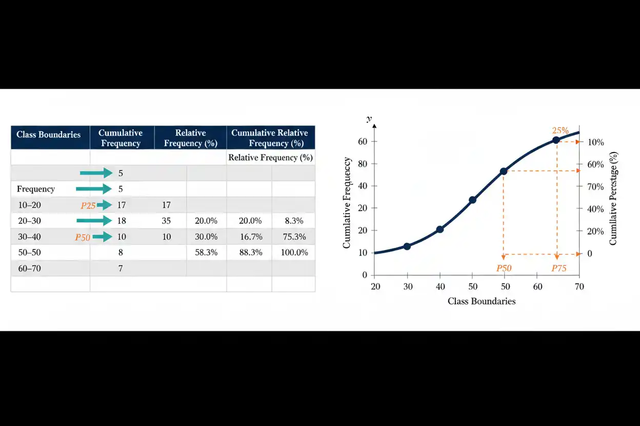
Cumulative frequency is the running total of frequencies in an ordered data set, showing how many observations fall at or below each value, category boundary, or class interval. Instead of describing only how often an individual value occurs, cumulative frequency progressively adds each new frequency to all frequencies that came before it, which makes the method particularly useful for identifying medians, quartiles, percentiles, proportions below thresholds, and the distribution of observations across ordered ranges. If ordinary frequencies are f₁, f₂, f₃, …, then the cumulative frequency at the kth position is the sum Fₖ = f₁ + f₂ + … + fₖ, and the final cumulative frequency must equal the total number of observations n when every observation has been included exactly once. The same idea can be converted into cumulative relative frequency by dividing each running total by n, producing values between 0 and 1, or cumulative percentages between 0% and 100%. Cumulative frequency tables can also be represented graphically with an ogive, an increasing curve that makes positional quantities such as the median or 75th percentile easier to estimate visually.
Cumulative frequency belongs to the broader framework of descriptive statistics within Statistics & Probability. It extends the information contained in a frequency distribution by answering not merely “how many observations occur here?” but “how many observations have accumulated up to this point?”
What Is Cumulative Frequency?
Cumulative frequency is the sum of a frequency and all frequencies preceding it in an ordered distribution.
Suppose ordinary frequencies are:
3, 5, 4, 2
The cumulative frequencies are calculated as:
3
3 + 5 = 8
3 + 5 + 4 = 12
3 + 5 + 4 + 2 = 14
Therefore:
Cumulative frequencies = 3, 8, 12, 14
The final result:
14
is the total number of observations.
Because the totals accumulate rather than decrease, an ordinary less-than-or-equal cumulative frequency sequence must be nondecreasing.
Cumulative Frequency Formula
If:
f₁, f₂, …, fₖ
are ordinary frequencies, then cumulative frequency at position k is:
Fₖ = Σᵢ₌₁ᵏ fᵢ
Equivalently:
F₁ = f₁
and for later positions:
Fₖ = Fₖ₋₁ + fₖ
This recursive form is often easiest for constructing a table manually.
For example, if:
F₃ = 12
and:
f₄ = 7
then:
F₄ = 12 + 7
= 19
The running-total interpretation and summation formula describe the same quantity.
Simple Cumulative Frequency Example
Suppose the observations are:
1, 1, 2, 2, 2, 3, 3, 4
First construct the ordinary frequencies:
| Value | Frequency |
|---|---|
| 1 | 2 |
| 2 | 3 |
| 3 | 2 |
| 4 | 1 |
Now calculate cumulative frequency:
| Value | Frequency | Cumulative Frequency |
|---|---|---|
| 1 | 2 | 2 |
| 2 | 3 | 5 |
| 3 | 2 | 7 |
| 4 | 1 | 8 |
The interpretation is immediate.
At or below:
2
there are:
5 observations.
At or below:
3
there are:
7 observations.
The final cumulative frequency equals:
n = 8.
Why Data Must Be Ordered
Cumulative frequency depends on order because the phrase “up to this point” must have numerical or ordinal meaning.
For numerical values, ordering is straightforward:
1, 2, 3, 4
For ordered categories, one might use:
Low, Medium, High
A cumulative total can then represent the number at or below each ordered level.
For unordered nominal categories such as:
Red, Blue, Green
there is no natural “less than or equal to” relationship unless an arbitrary ordering is imposed.
In that situation, ordinary frequencies are usually more meaningful than cumulative frequencies.
Frequency vs Cumulative Frequency
Frequency answers:
How many observations occur in this value or class?
Cumulative frequency answers:
How many observations occur in this value or class and all preceding ones?
Suppose:
| Score | Frequency | Cumulative Frequency |
|---|---|---|
| 10 | 4 | 4 |
| 20 | 6 | 10 |
| 30 | 5 | 15 |
At score 20:
Frequency = 6
means exactly six observations have score 20.
By contrast:
Cumulative frequency = 10
means ten observations have scores at or below 20.
Confusing these columns changes the statistical meaning substantially.
Running Total Method
The easiest manual approach is often to create a running total.
Suppose frequencies are:
6, 4, 8, 5, 2
Begin with:
F₁ = 6
Then:
F₂ = 6 + 4 = 10
F₃ = 10 + 8 = 18
F₄ = 18 + 5 = 23
F₅ = 23 + 2 = 25
Thus:
Cumulative frequencies = 6, 10, 18, 23, 25
The final total tells us:
n = 25.
Each cumulative frequency must be at least as large as the previous one because ordinary frequencies cannot be negative.
Cumulative Relative Frequency
Cumulative relative frequency converts a cumulative count into a proportion of the complete data set.
The formula is:
Cumulative relative frequency = Fₖ/n
where:
- Fₖ = cumulative frequency
- n = total number of observations
Suppose:
n = 50
and the cumulative frequency through one class is:
Fₖ = 35
Then:
Cumulative relative frequency = 35/50
= 0.70
Therefore:
70%
of observations fall at or below that value or class boundary.
Cumulative Percentage
A cumulative relative frequency can be converted into a percentage:
Cumulative percentage = (Fₖ/n) × 100%
If:
Fₖ = 18
and:
n = 24
then:
Cumulative percentage = (18/24) × 100%
= 75%
This indicates that:
75%
of observations lie at or below the relevant point.
The final cumulative percentage must be:
100%
when the table includes the complete data set.
Full Relative Frequency Example
Suppose:
| Value | Frequency |
|---|---|
| 1 | 5 |
| 2 | 8 |
| 3 | 4 |
| 4 | 3 |
Total:
n = 20
Cumulative frequencies are:
5, 13, 17, 20
Divide each by 20:
5/20 = 0.25
13/20 = 0.65
17/20 = 0.85
20/20 = 1.00
Therefore:
| Value | Frequency | Cumulative Frequency | Cumulative Relative Frequency |
|---|---|---|---|
| 1 | 5 | 5 | 0.25 |
| 2 | 8 | 13 | 0.65 |
| 3 | 4 | 17 | 0.85 |
| 4 | 3 | 20 | 1.00 |
The cumulative relative-frequency column ends at exactly:
1.00
or:
100%.
Cumulative Frequency for Grouped Data
Cumulative frequency is especially useful when numerical observations have been grouped into intervals.
Suppose:
| Interval | Frequency |
|---|---|
| 0–10 | 4 |
| 10–20 | 7 |
| 20–30 | 10 |
| 30–40 | 6 |
| 40–50 | 3 |
Calculate the running totals:
4
4 + 7 = 11
11 + 10 = 21
21 + 6 = 27
27 + 3 = 30
Therefore:
| Interval | Frequency | Cumulative Frequency |
|---|---|---|
| 0–10 | 4 | 4 |
| 10–20 | 7 | 11 |
| 20–30 | 10 | 21 |
| 30–40 | 6 | 27 |
| 40–50 | 3 | 30 |
The total number of observations is:
n = 30.
Interpreting Grouped Cumulative Frequency
In the grouped example:
Cumulative frequency through 20–30 = 21.
Under a conventional non-overlapping class interpretation, this means:
21 observations
lie below the upper boundary of the 20–30 class.
Similarly:
Cumulative frequency through 30–40 = 27
means:
27 observations
lie below the upper boundary of that class.
The exact wording should respect the class-boundary convention.
If intervals are written as:
20 ≤ x < 30
then cumulative frequency through that class represents observations with:
x < 30.
Less-Than Cumulative Frequency
A less-than cumulative frequency table accumulates observations from the lowest values upward.
For grouped intervals:
0–10
10–20
20–30
one can summarize:
Less than 10
Less than 20
Less than 30
Suppose frequencies are:
4, 7, 10.
Then:
Less than 10 → 4
Less than 20 → 11
Less than 30 → 21
This is the most common direction for cumulative frequency tables and produces an increasing sequence.
Greater-Than Cumulative Frequency
A greater-than cumulative frequency works in the opposite direction.
Instead of counting observations below successive boundaries, it counts observations at or above successive lower boundaries.
Suppose the total is:
30
and grouped frequencies are:
4, 7, 10, 6, 3.
Then a greater-than cumulative sequence can be:
At least 0 → 30
At least 10 → 26
At least 20 → 19
At least 30 → 9
At least 40 → 3
This sequence decreases because observations are progressively removed as the lower threshold rises.
The direction must therefore be identified before interpreting a cumulative-frequency table.
Recovering Ordinary Frequency From Cumulative Frequency
Ordinary frequencies can be recovered from successive cumulative totals.
If:
F₁ = 5
then:
f₁ = 5.
For later positions:
fₖ = Fₖ − Fₖ₋₁
Suppose cumulative frequencies are:
5, 12, 20, 24
Then:
f₁ = 5
f₂ = 12 − 5 = 7
f₃ = 20 − 12 = 8
f₄ = 24 − 20 = 4
Therefore:
Ordinary frequencies = 5, 7, 8, 4.
This inverse relationship is useful when only cumulative totals are supplied.
Recovering Frequency Example
Suppose:
| Value | Cumulative Frequency |
|---|---|
| 10 | 3 |
| 20 | 9 |
| 30 | 15 |
| 40 | 20 |
Find the ordinary frequencies.
For 10:
f₁ = 3
For 20:
f₂ = 9 − 3
= 6
For 30:
f₃ = 15 − 9
= 6
For 40:
f₄ = 20 − 15
= 5
Thus:
| Value | Frequency |
|---|---|
| 10 | 3 |
| 20 | 6 |
| 30 | 6 |
| 40 | 5 |
The frequencies sum to:
20
which matches the final cumulative frequency.
Cumulative Frequency and the Median
The median is the central ordered position.
For an odd number of observations:
Median position = (n + 1)/2
For even n, the usual sample median is based on the two central ordered positions:
n/2
and:
n/2 + 1.
Cumulative frequency helps identify the value or class containing those positions.
For example, if:
n = 21
then the median occupies position:
(21 + 1)/2 = 11.
Find the first cumulative frequency reaching or exceeding:
The corresponding value or class contains the sample median.
Median From a Discrete Frequency Table
Suppose:
| Value | Frequency | Cumulative Frequency |
|---|---|---|
| 1 | 4 | 4 |
| 2 | 5 | 9 |
| 3 | 7 | 16 |
| 4 | 4 | 20 |
Here:
n = 20.
The two central positions are:
10th and 11th.
Cumulative frequency reaches:
9
at value 2 and:
16
at value 3.
Therefore, both the 10th and 11th observations are:
3
so:
Median = 3.
Cumulative frequency allows the median to be located without expanding the entire data set.
Cumulative Frequency and Quartiles
Quartiles divide ordered data into broad positional sections.
Conceptually:
Q₁ ≈ 25th percentile
Q₂ = median ≈ 50th percentile
Q₃ ≈ 75th percentile.
A cumulative-frequency table can identify where these positions occur.
For example, with:
n = 100
the rough quartile positions correspond to cumulative frequencies near:
25
50
The exact finite-sample quartile convention can differ, but cumulative frequency provides the positional framework needed to locate the quartile values or classes.
Cumulative Frequency and the Five-Number Summary
The five-number summary contains:
Minimum
Q₁
Median
Q₃
Maximum
A cumulative-frequency table can help locate all three central positional quantities:
Q₁
Median
Q₃.
The minimum and maximum are obtained from the ends of the observed distribution.
Thus cumulative frequency provides one route from a frequency table to the positional summaries used in quartile-based descriptive analysis.
Cumulative Frequency and Percentiles
A percentile identifies a value below which a specified percentage of observations lie.
For the kth percentile, the target cumulative proportion is approximately:
k/100.
For example, the:
90th percentile
corresponds to cumulative proportion:
0.90.
If:
n = 200
the corresponding cumulative position is roughly:
0.90(200)
= 180.
One then identifies where the cumulative frequency reaches the relevant percentile position, applying the chosen percentile convention.
Grouped data may require interpolation within the containing class.
Percentile Example
Suppose:
n = 50
and cumulative frequencies are:
| Value | Cumulative Frequency |
|---|---|
| 10 | 8 |
| 20 | 20 |
| 30 | 36 |
| 40 | 45 |
| 50 | 50 |
The 80th-percentile position is approximately:
0.80(50)
= 40.
Cumulative frequency is:
36
at value 30 and:
45
at value 40.
Therefore, the 80th-percentile observation lies within the set represented by value:
40
for this discrete table.
With grouped continuous data, interpolation may be used instead.
Grouped Median Formula
For grouped continuous data, the median is often estimated using:
Median ≈ L + [(n/2 − F_prev)/f_m]h
where:
- L = lower class boundary of the median class
- n = total frequency
- F_prev = cumulative frequency before the median class
- f_m = frequency of the median class
- h = class width
This formula assumes observations are distributed approximately uniformly within the median class for interpolation purposes.
It is therefore an estimate, not an exact reconstruction of the unknown raw observations.
Grouped Median Example
Suppose:
| Class | Frequency | Cumulative Frequency |
|---|---|---|
| 0–10 | 4 | 4 |
| 10–20 | 6 | 10 |
| 20–30 | 10 | 20 |
| 30–40 | 8 | 28 |
| 40–50 | 2 | 30 |
Total:
n = 30
The median position is:
n/2 = 15.
The first cumulative frequency reaching or exceeding 15 is:
20
in the:
20–30
class.
Therefore, this is the median class.
Using:
L = 20
F_prev = 10
f_m = 10
h = 10
we get:
Median ≈ 20 + (15 − 10)/10
= 20 + 5
= 25
So the grouped median is estimated as:
Grouped Quartile Formula
A similar interpolation approach can be used for grouped quartiles.
For the kth quartile position q:
Q ≈ L + [(q − F_prev)/f]h
where q is the required cumulative-frequency position.
For Q₁:
q ≈ n/4
For Q₂:
q ≈ n/2
For Q₃:
q ≈ 3n/4.
The exact positional convention can vary, but the cumulative frequencies identify the class containing the desired quantile.
What Is an Ogive?
An ogive is a graph of cumulative frequency or cumulative relative frequency.
For a less-than ogive:
- the horizontal axis shows values or upper class boundaries;
- the vertical axis shows cumulative frequency, proportion, or percentage.
Because cumulative frequency cannot decrease in a less-than table, the ogive rises or remains flat as x increases.
The final point reaches:
n
for cumulative count,
1
for cumulative relative frequency,
or:
100%
for cumulative percentage.
An ogive provides a visual representation of the cumulative distribution.
How to Draw an Ogive
Suppose the grouped table is:
| Class | Cumulative Frequency |
|---|---|
| 0–10 | 4 |
| 10–20 | 11 |
| 20–30 | 21 |
| 30–40 | 27 |
| 40–50 | 30 |
Plot cumulative frequency against upper class boundaries:
(10, 4)
(20, 11)
(30, 21)
(40, 27)
(50, 30)
A starting point at the lowest class boundary with cumulative frequency zero may also be included:
(0, 0).
Connecting the points gives the ogive.
The curve can then be used to estimate medians, quartiles, and proportions below chosen thresholds.
Reading a Median From an Ogive
Suppose total frequency is:
n = 100.
The median corresponds to cumulative frequency:
On the vertical axis, locate:
Move horizontally until reaching the ogive, then move vertically down to the x-axis.
The corresponding x-value provides an approximate median.
The same method can estimate Q₁ using cumulative frequency 25 and Q₃ using cumulative frequency 75.
The accuracy depends on the grouped representation and graphical scale.
Reading Percentages From an Ogive
If the vertical axis displays cumulative percentage, percentile interpretation becomes especially direct.
To estimate the 90th percentile:
- locate:90%
on the vertical axis; - move horizontally to the curve;
- move down to the horizontal axis.
The resulting x-value estimates the point below which approximately 90% of observations fall.
Conversely, to estimate the proportion below a specific x-value, move upward from x to the curve and then horizontally to the cumulative-percentage axis.
Cumulative Frequency vs Frequency Distribution
A frequency distribution emphasizes local counts.
For example:
10–20 → 7 observations.
A cumulative-frequency distribution emphasizes accumulation:
At or below 20 → 11 observations.
Ordinary frequencies are better for seeing where observations are concentrated in specific categories or intervals.
Cumulative frequencies are better for threshold and positional questions.
Both can be generated from the same underlying data and should be regarded as complementary summaries.
Cumulative Frequency vs Relative Frequency
Relative frequency for one class is:
fₖ/n.
Cumulative relative frequency is:
Fₖ/n.
Suppose:
n = 40
and one class has:
f = 6
while cumulative frequency through that class is:
F = 30.
Then:
Relative frequency = 6/40
= 15%
while:
Cumulative relative frequency = 30/40
= 75%.
The first tells us how much of the data belongs specifically to that class.
The second tells us how much of the data lies in that class or below it.
Cumulative Frequency and Box Plots
A box plot displays quartiles and median graphically.
Cumulative frequency can help locate those same positional values before the box plot is constructed.
For example:
25% cumulative position → Q₁
50% cumulative position → Median
75% cumulative position → Q₃.
Thus, cumulative distributions and box plots encode related positional information in different forms.
The cumulative-frequency display retains more detail about how observations build up across the complete range, while the box plot compresses the distribution into a few key landmarks.
Cumulative Frequency and Confidence Intervals
A confidence interval addresses uncertainty about a population parameter, whereas cumulative frequency describes observed counts or proportions up to thresholds.
For example, a sample cumulative-frequency table can show that:
70%
of observed values are at or below 50.
That is a descriptive sample result.
Estimating the corresponding population proportion with quantified sampling uncertainty requires an inferential interval procedure.
Cumulative frequency and confidence intervals therefore operate at different levels: one summarizes the observed distribution, while the other quantifies uncertainty about a population quantity.
Cumulative Frequency and Coefficient of Variation
The coefficient of variation summarizes relative mean-centered spread with:
CV = s/x̄
for a common sample form.
Cumulative frequency instead preserves ordered positional information.
Two data sets can have the same:
mean
and:
standard deviation
and therefore the same coefficient of variation, yet different cumulative-frequency patterns because their observations are distributed differently.
This is another reason a single dispersion statistic cannot completely describe a distribution.
Increasing Property of Cumulative Frequency
For an ordinary less-than cumulative distribution:
F₁ ≤ F₂ ≤ F₃ ≤ … ≤ Fₖ.
This follows because:
Fₖ = Fₖ₋₁ + fₖ
and:
fₖ ≥ 0.
If a cumulative-frequency table decreases from one row to the next, either:
- the table is using a greater-than direction;
- the rows are not ordered correctly;
- or a calculation error has occurred.
Checking monotonicity is therefore a useful quality-control step.
Final Cumulative Frequency Must Equal n
For a complete less-than cumulative-frequency distribution:
F_final = Σfᵢ
and:
Σfᵢ = n.
Therefore:
F_final = n.
If ordinary frequencies sum to:
73
but the final cumulative frequency is:
71
there is a calculation or data-entry problem.
Likewise, final cumulative relative frequency should equal:
1
and final cumulative percentage should equal:
100%
apart from tiny discrepancies caused by rounded displayed percentages.
Missing Categories With Zero Frequency
An ordered value can have frequency zero but cumulative frequency remains unchanged.
Suppose:
| Value | Frequency |
|---|---|
| 1 | 3 |
| 2 | 0 |
| 3 | 5 |
Then cumulative frequencies are:
3, 3, 8.
The cumulative total does not decrease at value 2.
On an ogive or step-style cumulative graph, the distribution remains flat through a zero-frequency region.
Such flat sections indicate intervals where no new observations accumulate.
Repeated Values
Repeated values are naturally handled by frequency tables.
Suppose:
5
appears eight times.
Then its ordinary frequency is:
If cumulative frequency before value 5 is:
20
then cumulative frequency at value 5 becomes:
20 + 8
= 28.
There is no need to list each repeated observation separately.
This is one reason cumulative-frequency tables are efficient for discrete data containing many repetitions.
Cumulative Frequency for Large Data Sets
For very large data sets, cumulative distributions can summarize thresholds efficiently.
Suppose a data set contains:
1,000,000
observations.
A cumulative table can answer questions such as:
How many values are ≤ 100?
What percentage are below 250?
Where is the 95th percentile?
without requiring a reader to inspect the entire data set.
Computationally, cumulative totals can be calculated efficiently after values or classes have been ordered.
Cumulative Distribution Function Connection
In probability theory, cumulative relative frequency is closely related to the empirical cumulative distribution function.
For observed data:
x₁, x₂, …, xₙ
the empirical CDF can be written:
Fₙ(x) = Number of observations ≤ x / n
Equivalently:
Fₙ(x) = (1/n)ΣI(xᵢ ≤ x)
where I is an indicator function.
Thus, empirical cumulative relative frequency is essentially the empirical probability distribution accumulated up to x.
As x increases beyond the largest observation:
Fₙ(x) = 1.
Properties of an Empirical Cumulative Distribution
An empirical cumulative distribution function is:
- nondecreasing;
- bounded between 0 and 1;
- equal to 0 below the minimum observation;
- equal to 1 at or above the maximum observation;
- step-shaped for finite data.
Each observation contributes a jump of:
1/n
when all observed values are distinct.
Repeated values create larger jumps because several observations accumulate at the same x-value.
This formalizes the intuitive running-total idea behind cumulative relative frequency.
Cumulative Frequency and Probability
A sample cumulative proportion can estimate a population cumulative probability.
Suppose:
800
of:
1,000
sample observations satisfy:
X ≤ 50.
Then the empirical cumulative proportion is:
800/1000
= 0.80.
This is a sample estimate of the population quantity:
P(X ≤ 50).
However, the sample result is subject to sampling variability unless the observations constitute the complete population of interest.
Statistical inference is required to quantify uncertainty about the population probability.
Comparing Two Cumulative Distributions
Cumulative relative-frequency curves can compare two samples over their entire numerical range.
Suppose Group A’s cumulative curve lies consistently above Group B’s curve over much of the domain.
At a given threshold x, this means a larger fraction of Group A observations fall at or below x.
Such comparisons can reveal distributional shifts that are not captured by means alone.
However, visual separation does not automatically establish statistical significance.
Formal distributional comparison requires an appropriate inferential method.
Cumulative Frequency and Sample Size
Raw cumulative frequency depends directly on sample size.
Suppose Sample A has:
n = 100
and Sample B has:
n = 10,000.
Comparing cumulative counts directly can be misleading because B will naturally reach much larger numbers.
Cumulative relative frequencies or percentages put both samples on a common:
0 to 1
or:
0% to 100%
scale.
This makes distributional comparison more meaningful when sample sizes differ.
Grouped Data and Information Loss
When raw values are replaced with class intervals, some information is lost.
Suppose an interval:
20–30
contains:
10 observations.
The cumulative table tells us how many observations have accumulated through that class, but not exactly where those ten observations lie within the interval.
Therefore, grouped median or percentile calculations often interpolate between class boundaries.
Those interpolated results should be understood as estimates based on within-class assumptions.
Narrower classes generally preserve more positional information but produce larger tables.
Unequal Class Widths
Cumulative frequency itself can be calculated with unequal class widths without difficulty because it counts observations rather than comparing bar heights.
Suppose classes are:
0–5
5–20
20–100.
One can still add their frequencies cumulatively.
However, ordinary histograms require special care with unequal class widths because frequency density rather than raw frequency may determine bar height.
Cumulative-frequency totals do not need that correction, although interpretation of broad intervals remains less precise.
Class Boundaries Matter
For continuous grouped data, classes must be defined so that every observation belongs to one and only one interval.
For example:
0 ≤ x < 10
10 ≤ x < 20
avoids ambiguity at:
x = 10.
If classes are written casually as:
0–10
10–20
the boundary convention should be understood before interpreting cumulative counts exactly.
This becomes especially important when the table is used to estimate thresholds or quantiles.
Cumulative Frequency With Open-Ended Classes
An open-ended interval such as:
50+
can be included as the final class of a cumulative-frequency table.
Its final cumulative frequency still equals:
n.
However, precise calculations involving the upper tail can become difficult because the maximum or class width is unknown.
For example, estimating a grouped mean from an open-ended final class requires additional assumptions.
Cumulative counts themselves remain valid because they require only the number of observations, not the exact values inside the class.
Common Cumulative Frequency Mistakes
A common mistake is writing the original frequency in the cumulative-frequency column rather than adding it to the preceding total.
Another error is starting cumulative totals before sorting numerical values or intervals into ascending order.
Analysts may also confuse cumulative frequency with cumulative percentage. A count of:
30
is not the same as:
30%
unless the total sample happens to be 100.
Another mistake is assuming a cumulative-frequency table for unordered nominal categories has natural statistical meaning.
For grouped data, using ambiguous or overlapping intervals can cause observations to be counted incorrectly.
It is also incorrect to treat the final cumulative frequency as anything other than the total count n in a complete less-than table.
Finally, interpolated grouped medians and percentiles should not be presented as exact raw-data results when the exact positions of observations within classes are unknown.
How to Calculate Cumulative Frequency Step by Step
First, arrange the values or class intervals in ascending order.
Next record the ordinary frequency for each value or interval.
Use the first ordinary frequency as the first cumulative frequency:
F₁ = f₁.
For every subsequent row, add the new ordinary frequency to the previous cumulative total:
Fₖ = Fₖ₋₁ + fₖ.
Continue until every class has been included.
Check that:
Final cumulative frequency = n.
If cumulative relative frequency is required, divide each cumulative count by n. If cumulative percentage is required, multiply those proportions by 100.
Full Worked Cumulative Frequency Example
Suppose test scores are grouped as:
| Score Range | Frequency |
|---|---|
| 0–10 | 3 |
| 10–20 | 5 |
| 20–30 | 9 |
| 30–40 | 7 |
| 40–50 | 4 |
| 50–60 | 2 |
Step 1: Find Total Frequency
n = 3 + 5 + 9 + 7 + 4 + 2
n = 30
Step 2: Calculate Cumulative Frequencies
First class:
F₁ = 3
Second:
F₂ = 3 + 5
= 8
Third:
F₃ = 8 + 9
= 17
Fourth:
F₄ = 17 + 7
= 24
Fifth:
F₅ = 24 + 4
= 28
Sixth:
F₆ = 28 + 2
= 30
Therefore:
| Score Range | Frequency | Cumulative Frequency |
|---|---|---|
| 0–10 | 3 | 3 |
| 10–20 | 5 | 8 |
| 20–30 | 9 | 17 |
| 30–40 | 7 | 24 |
| 40–50 | 4 | 28 |
| 50–60 | 2 | 30 |
Add Cumulative Percentages
Divide each cumulative frequency by:
30
and multiply by 100.
For the first class:
3/30 × 100 = 10%
Second:
8/30 × 100 ≈ 26.67%
Third:
17/30 × 100 ≈ 56.67%
Fourth:
24/30 × 100 = 80%
Fifth:
28/30 × 100 ≈ 93.33%
Final:
30/30 × 100 = 100%
The full table becomes:
| Score Range | Frequency | Cumulative Frequency | Cumulative % |
|---|---|---|---|
| 0–10 | 3 | 3 | 10.00% |
| 10–20 | 5 | 8 | 26.67% |
| 20–30 | 9 | 17 | 56.67% |
| 30–40 | 7 | 24 | 80.00% |
| 40–50 | 4 | 28 | 93.33% |
| 50–60 | 2 | 30 | 100.00% |
Interpret the Worked Example
The table shows that:
17 of 30 observations
fall below the upper boundary of the 20–30 class.
As a percentage:
56.67%
of observations have accumulated through that class.
Similarly:
24 of 30
or:
80%
have accumulated through the 30–40 class.
Only:
6 observations
remain above that point because:
30 − 24 = 6.
Cumulative frequency therefore allows both below-threshold and remaining-above-threshold counts to be derived easily.
Estimate the Median Class
The total is:
n = 30
so the median position is around:
n/2 = 15.
The cumulative frequencies are:
3, 8, 17, 24, 28, 30.
The first cumulative frequency that reaches or exceeds 15 is:
Therefore, the median lies in the:
20–30
class.
Using grouped interpolation:
L = 20
F_prev = 8
f_m = 9
h = 10
Therefore:
Median ≈ 20 + (15 − 8)/9
= 20 + (7/9)(10)
≈ 20 + 7.78
≈ 27.78
Thus, under the standard within-class interpolation assumption:
Grouped median ≈ 27.78.
Estimate the 80th Percentile
The 80th-percentile position is:
0.80(30)
= 24.
Cumulative frequency reaches:
24
at the end of the:
30–40
class.
Therefore, under this grouped structure, the 80th percentile is approximately at the upper boundary:
This agrees with the cumulative percentage table, which shows:
80%
through that class.
The example demonstrates how cumulative frequency directly supports percentile interpretation.
How to Report Cumulative Frequency
A clear descriptive statement identifies both the threshold and the accumulated count or percentage.
For example:
“Twenty-four of 30 observations, or 80%, were below the upper boundary of the 30–40 class.”
For discrete data:
“Seventeen observations had values at or below 3.”
If the table uses greater-than rather than less-than accumulation, state that explicitly.
When grouped interpolation is used to estimate a median or percentile, identify the result as an estimate rather than implying that the exact raw-data quantile was observed.
Frequently Asked Questions About Cumulative Frequency
What is cumulative frequency?
Cumulative frequency is the running total of ordinary frequencies across ordered values or class intervals.
What is the cumulative frequency formula?
Fₖ = Σᵢ₌₁ᵏ fᵢ
What is the recursive cumulative frequency formula?
Fₖ = Fₖ₋₁ + fₖ
What is the first cumulative frequency?
It equals the first ordinary frequency:
F₁ = f₁
What should the final cumulative frequency equal?
For a complete less-than table:
Final cumulative frequency = n
Can cumulative frequency decrease?
A less-than cumulative frequency should not decrease. A greater-than cumulative distribution can decrease as the threshold rises.
What is cumulative relative frequency?
Fₖ/n
It expresses cumulative frequency as a proportion of the total.
What is cumulative percentage?
(Fₖ/n) × 100%
What should the final cumulative relative frequency equal?
1
What should the final cumulative percentage equal?
100%
What is the difference between frequency and cumulative frequency?
Frequency counts observations in one value or class. Cumulative frequency counts observations in that value or class plus all preceding values or classes.
How do you recover ordinary frequency from cumulative frequency?
For later rows:
fₖ = Fₖ − Fₖ₋₁
Do data need to be sorted first?
Yes. Cumulative frequency requires a meaningful order.
Can cumulative frequency be used for nominal categories?
Usually not meaningfully unless the categories have a genuine order.
Can cumulative frequency be used for ordinal data?
Yes, when the category ordering is meaningful.
Can cumulative frequency be used for continuous data?
Yes, usually through grouped class intervals or the empirical cumulative distribution.
What is an ogive?
An ogive is a graph of cumulative frequency, cumulative relative frequency, or cumulative percentage against ordered values or class boundaries.
Does an ogive always increase?
A less-than ogive is nondecreasing. A greater-than cumulative curve generally decreases.
How do you find the median from cumulative frequency?
Locate the cumulative position around the middle of the ordered data and identify the value or class where the cumulative frequency reaches that position.
How do you find Q₁?
Locate approximately the:
25%
cumulative position.
How do you find Q₃?
Locate approximately the:
75%
cumulative position.
How do you find a percentile?
Locate the corresponding cumulative proportion or cumulative-frequency position, using the chosen percentile convention.
What is the median class?
It is the class interval containing the median position.
What is the grouped median formula?
A common interpolation formula is:
Median ≈ L + [(n/2 − F_prev)/f_m]h
Is a grouped median exact?
Usually not. It is estimated because exact observation locations within the median class are unknown.
How does cumulative frequency relate to a five-number summary?
It can help locate Q₁, median, and Q₃, which form the central three values of the five-number summary.
How does cumulative frequency relate to a box plot?
Quartiles identified through ordered or cumulative information provide the box boundaries and median used in a box plot.
How is cumulative frequency different from a confidence interval?
Cumulative frequency describes observed distribution counts, while a confidence interval quantifies uncertainty about an unknown population parameter.
Can cumulative frequencies be converted to probabilities?
Cumulative relative frequencies can estimate cumulative probabilities from sample data, but population inference remains subject to sampling uncertainty.
What is an empirical cumulative distribution function?
It is the fraction of observations at or below x:
Fₙ(x) = Number of observations ≤ x / n
Is cumulative frequency affected by sample size?
Raw cumulative counts are. Cumulative proportions and percentages make comparisons across different sample sizes easier.
Can a class have zero frequency?
Yes. The cumulative frequency then remains unchanged through that class.
Can cumulative frequency be calculated with unequal class widths?
Yes. It is based on counts, although broad unequal intervals can reduce positional detail.
What happens with an open-ended final class?
Its cumulative frequency can still reach n, although some calculations requiring exact upper boundaries may become difficult.
Why is cumulative frequency useful?
It quickly answers threshold questions, reveals cumulative proportions, and helps locate medians, quartiles, percentiles, and other ordered positions.
What is the most important rule when calculating cumulative frequency?
Order the values or intervals correctly, add frequencies progressively without skipping or double-counting observations, and verify that the final cumulative total equals the complete number of observations.




