

Confidence Interval: Definition, Formula & Example

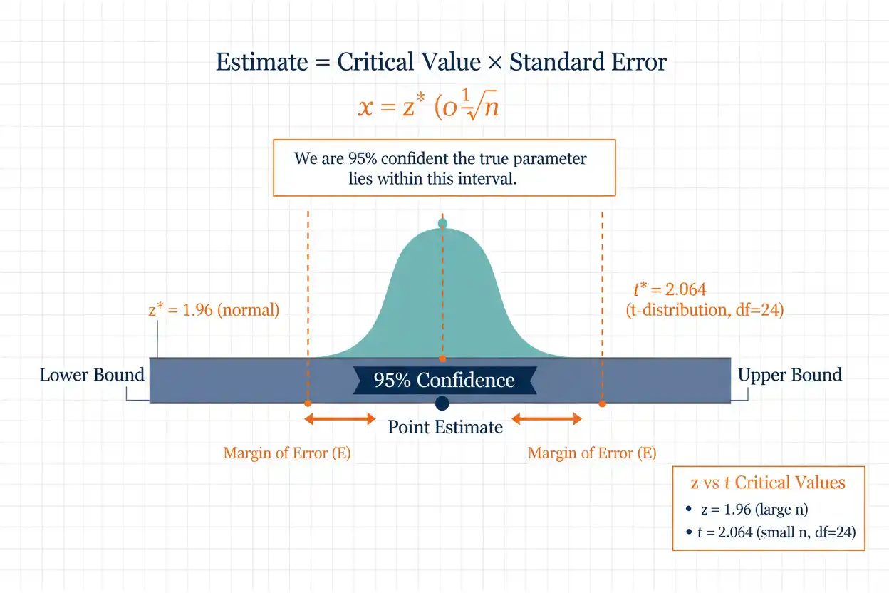
A confidence interval is a range of plausible values for an unknown population parameter constructed from sample data using a statistical procedure with a specified long-run coverage rate. Rather than reporting only a single point estimate such as a sample mean or sample proportion, a confidence interval combines that estimate with information about sampling uncertainty, producing lower and upper bounds that show how precisely the parameter has been estimated under the assumptions of the method. The general structure is estimate ± critical value × standard error, where the estimate identifies the center of the interval, the standard error measures how much the estimator would vary across repeated samples, and the critical value determines how much of the reference sampling distribution the procedure is designed to cover. A 95% confidence interval does not ordinarily mean there is a 95% probability that the fixed population parameter lies inside one particular interval after it has been calculated; instead, it means that if the same sampling and interval-construction procedure were repeated many times under the model assumptions, approximately 95% of the resulting intervals would contain the true parameter. Confidence intervals therefore provide more information than a point estimate alone because they show both estimated magnitude and statistical precision, while their reliability still depends on sampling design, model assumptions, independence, sample size, variability, and the suitability of the standard-error calculation.
Confidence intervals connect descriptive summaries such as the arithmetic mean with inferential reasoning about unknown population quantities. Within descriptive statistics and the broader Statistics & Probability framework, they mark an important transition from describing what was observed to quantifying how uncertain a population estimate remains.
What Is a Confidence Interval?
A confidence interval is an interval estimate for an unknown population parameter.
Examples of parameters that can have confidence intervals include:
Population mean: μ
Population proportion: p
Difference between means: μ₁ − μ₂
Difference between proportions: p₁ − p₂
Regression coefficient: β
The interval is calculated from sample data.
A typical result might be:
95% CI = (48.2, 53.6)
This means the statistical procedure has produced a lower bound of:
48.2
and an upper bound of:
53.6.
The width of that interval communicates uncertainty about the parameter estimate.
General Confidence Interval Formula
Many confidence intervals have the general structure:
Confidence interval = Estimate ± Margin of error
where:
Margin of error = Critical value × Standard error
Therefore:
Confidence interval = Estimate ± Critical value × Standard error
The two endpoints are:
Lower bound = Estimate − Critical value × SE
Upper bound = Estimate + Critical value × SE
This simple structure appears throughout classical statistics, although the exact estimate, standard error, critical value, and reference distribution differ among problems.
Parts of a Confidence Interval
A confidence interval usually contains four main statistical components.
The point estimate is the sample-based estimate of the population parameter.
The standard error measures the sampling variability of that estimate.
The critical value determines how far the interval extends in standard-error units.
The confidence level specifies the long-run coverage target of the interval procedure.
For example:
x̄ = 100
SE = 4
z* = 1.96
produces:
100 ± 1.96(4)
so the margin of error is:
7.84
and the interval is:
(92.16, 107.84)
Point Estimate
A point estimate is one sample-based value used to estimate a population parameter.
For a population mean μ, the sample mean:
x̄
is a common point estimator.
For a population proportion p, the sample proportion:
p̂
is a common point estimator.
Suppose:
x̄ = 75
The number 75 is the point estimate.
It provides no direct indication of how precisely μ has been estimated.
A confidence interval adds that uncertainty information.
Standard Error
A standard error is the standard deviation of an estimator’s sampling distribution or an estimate of that quantity.
For a sample mean with known population standard deviation σ:
SE(X̄) = σ/√n
If σ is unknown, a common estimated standard error is:
SÊ(X̄) = s/√n
For a sample proportion:
SE(p̂) = √[p(1−p)/n]
although p is unknown and practical confidence-interval methods use an estimated or method-specific standard error.
Smaller standard errors create narrower confidence intervals when the confidence level and method remain unchanged.
Margin of Error
The margin of error is:
E = Critical value × Standard error
For example, suppose:
z* = 1.96
and:
SE = 3
Then:
E = 1.96(3)
E = 5.88
If the point estimate is:
50
the interval is:
50 ± 5.88
or:
(44.12, 55.88)
The margin of error represents the distance from the point estimate to either endpoint in a symmetric interval.
Confidence Level
The confidence level describes the long-run coverage probability of the interval procedure under its assumptions.
Common confidence levels include:
90%
95%
99%
For a 95% confidence procedure, hypothetical repetition means that approximately:
95%
of intervals generated by the same method would contain the true parameter, while approximately:
5%
would fail to contain it.
The confidence level describes a property of the procedure.
It is not ordinarily a probability assigned to the fixed parameter after the particular sample has been observed.
What Does 95% Confidence Mean?
Suppose a study produces:
95% CI = (20, 30)
Under the frequentist interpretation, the true parameter is treated as fixed.
Before sampling, the endpoints are random because different samples would produce different intervals.
If the sampling process and interval method were repeated many times, approximately:
95%
of those intervals would contain the true parameter.
Once one interval has been calculated, it either contains the parameter or it does not.
The 95% refers to the reliability of the method over repeated sampling.
What a 95% Confidence Interval Does Not Mean
A frequentist 95% confidence interval is commonly misinterpreted as:
“There is a 95% probability the true parameter is inside this interval.”
That statement assigns probability directly to a fixed parameter, which is not the ordinary frequentist interpretation.
It is also incorrect to say:
“95% of observations lie inside the confidence interval.”
A confidence interval concerns uncertainty about a parameter, not the distribution of individual observations.
Likewise, it does not mean:
“95% of future sample means will fall inside this particular interval.”
Different predictive and sampling-distribution questions require different calculations.
Confidence Interval for a Mean With Known σ
When population standard deviation σ is known and the sampling distribution of the mean is normal or appropriately approximated by normality, a confidence interval for μ is:
x̄ ± z*σ/√n
where:
- x̄ = sample mean
- z* = standard normal critical value
- σ = known population standard deviation
- n = sample size
For a 95% interval:
z* ≈ 1.96
Therefore:
95% CI = x̄ ± 1.96σ/√n
under the applicable assumptions.
Known-σ Mean Example
Suppose:
x̄ = 80
σ = 12
n = 36
The standard error is:
SE = 12/√36
= 12/6
= 2
For a 95% confidence interval:
z* = 1.96
The margin of error is:
E = 1.96(2)
= 3.92
Therefore:
CI = 80 ± 3.92
giving:
Lower bound = 76.08
Upper bound = 83.92
Thus:
95% CI = (76.08, 83.92)
Interpreting the Mean Example
The sample mean is:
80
and the confidence interval extends approximately:
3.92 units
on either side.
The estimate therefore indicates a population mean plausibly represented, under the procedure, by values between approximately:
76.08 and 83.92.
A value near the center is more consistent with the point estimate than one near an endpoint in an informal descriptive sense, but the ordinary confidence interval itself is not a posterior probability distribution over μ.
Its main inferential statement concerns the repeated-sampling coverage of the interval-generating procedure.
Confidence Interval for a Mean When σ Is Unknown
Population standard deviation is often unknown.
For a sample from a normal population, the classical confidence interval uses the sample standard deviation s and Student’s t distribution:
x̄ ± t* s/√n
where:
df = n − 1
The t critical value is larger than the corresponding standard-normal value for finite degrees of freedom because estimating σ adds uncertainty.
As n becomes large, the t distribution approaches the standard normal distribution.
t-Based Mean Confidence Interval Example
Suppose:
n = 25
x̄ = 52
s = 10
For a 95% interval:
df = 25 − 1
df = 24
The relevant critical value is approximately:
t* = 2.064
Calculate the standard error:
SE = 10/√25
= 2
Margin of error:
E = 2.064(2)
= 4.128
Therefore:
CI = 52 ± 4.128
giving:
95% CI ≈ (47.87, 56.13)
Why the t Interval Is Wider
If the same example incorrectly used:
z* = 1.96
the margin would be:
1.96(2)
= 3.92
The t-based margin is:
4.128
which is slightly larger.
The difference accounts for uncertainty in estimating the population standard deviation.
With much smaller samples, the difference between t and z critical values is more substantial.
With very large samples, the two intervals become nearly identical numerically.
Degrees of Freedom
For a one-sample t confidence interval:
df = n − 1
Degrees of freedom affect the critical value.
For example, the approximate 95% two-sided critical values are:
df = 4 → t* ≈ 2.776
df = 10 → t* ≈ 2.228
df = 30 → t* ≈ 2.042
df → ∞ → t* ≈ 1.960
Smaller samples require wider intervals because estimated variability is itself more uncertain.
Common Standard Normal Critical Values
Frequently used z critical values include:
| Confidence Level | Critical Value z* |
|---|---|
| 80% | 1.282 |
| 90% | 1.645 |
| 95% | 1.960 |
| 98% | 2.326 |
| 99% | 2.576 |
Higher confidence levels use larger critical values.
Therefore, for the same point estimate and standard error:
99% CI is wider than 95% CI
and:
95% CI is wider than 90% CI.
Greater coverage confidence requires accepting less precision in the form of a wider interval.
Why Higher Confidence Produces a Wider Interval
Suppose:
Estimate = 100
SE = 5
For 90% confidence:
E = 1.645(5)
= 8.225
so:
90% CI = (91.775, 108.225)
For 95% confidence:
E = 1.96(5)
= 9.8
so:
95% CI = (90.2, 109.8)
For 99% confidence:
E = 2.576(5)
= 12.88
so:
99% CI = (87.12, 112.88)
Capturing a larger central portion of the reference sampling distribution requires extending farther from the estimate.
Confidence Level vs Precision
Confidence and precision trade off when sample size and variability are fixed.
Higher confidence:
increases critical value
and therefore:
increases interval width.
Lower confidence:
decreases critical value
and therefore:
decreases interval width.
Neither is inherently superior.
The selected confidence level should reflect the inferential purpose and consequences of uncertainty rather than being chosen solely to produce a narrow interval.
Sample Size and Confidence Interval Width
For a mean:
SE = σ/√n
or approximately:
s/√n.
Therefore, interval width decreases approximately as:
1/√n.
Suppose:
σ = 20.
At:
n = 25
we have:
SE = 20/5
= 4.
At:
n = 100
we have:
SE = 20/10
= 2.
Quadrupling sample size halves the standard error and therefore approximately halves the margin of error when the critical value is unchanged.
Why Doubling Sample Size Does Not Halve the Margin
Because standard error follows:
1/√n
doubling n changes the standard error by:
1/√2
which is approximately:
0.707.
Therefore, doubling sample size reduces the margin of error by roughly:
29.3%
rather than 50%.
To halve the standard error, sample size must generally be multiplied by:
This square-root relationship is fundamental to sample-size planning.
Variability and Interval Width
Greater variability produces wider confidence intervals.
For a sample mean:
SE = s/√n.
If:
s = 5
and:
n = 100
then:
SE = 0.5.
If:
s = 20
with the same n:
SE = 2.
The second interval is four times wider for the same critical value.
A highly variable population therefore requires more data to estimate its mean with the same precision.
Confidence Interval and Coefficient of Variation
The coefficient of variation measures standard deviation relative to the mean, whereas confidence-interval width depends on the standard error of the estimator.
Two groups can have different coefficients of variation and therefore very different relative dispersion, yet their confidence intervals also depend strongly on sample size.
For example, a group with high relative variability can still have a narrow confidence interval for its mean if n is enormous.
CV describes observation-level relative spread.
A confidence interval describes uncertainty about a population parameter.
These concepts should not be treated interchangeably.
Confidence Interval for a Population Proportion
For a sample proportion:
p̂ = x/n
a simple large-sample normal approximation is often written:
p̂ ± z*√[p̂(1−p̂)/n]
This is commonly known as the Wald interval.
Although easy to calculate, it can perform poorly when:
- n is small;
- p̂ is close to 0;
- p̂ is close to 1.
Alternative intervals such as the Wilson interval often provide better coverage behavior.
Therefore, the simple formula is useful for understanding structure but should not automatically be treated as the best method in every proportion problem.
Simple Proportion Interval Example
Suppose:
x = 120
successes occur in:
n = 200
observations.
Then:
p̂ = 120/200
= 0.60
The estimated standard error is:
SE ≈ √[(0.60)(0.40)/200]
= √(0.24/200)
= √0.0012
≈ 0.03464
For a 95% interval:
E = 1.96(0.03464)
≈ 0.0679
Therefore, the simple normal interval is:
0.60 ± 0.0679
or approximately:
(0.532, 0.668)
Thus, the estimated population proportion is 60%, with this approximate interval extending from 53.2% to 66.8%.
Why a Proportion Interval Can Stay Inside 0 and 1
A population proportion must satisfy:
0 ≤ p ≤ 1.
The simple Wald formula can sometimes generate endpoints below 0 or above 1, especially with small samples or proportions near the boundaries.
For example, an interval such as:
(−0.04, 0.20)
contains an impossible negative proportion.
This is one reason improved methods such as Wilson intervals are often preferred.
A confidence-interval method should respect the mathematical structure of the parameter whenever possible.
Difference Between Two Means
For two independent sample means, the parameter of interest can be:
μ₁ − μ₂.
The point estimate is:
x̄₁ − x̄₂.
When population variances are not assumed equal, an estimated standard error is:
SE = √(s₁²/n₁ + s₂²/n₂)
A Welch confidence interval has the form:
(x̄₁ − x̄₂) ± t*SE
where t* uses appropriate Welch-Satterthwaite degrees of freedom.
An interval containing:
0
indicates that a zero difference remains compatible with the corresponding two-sided confidence procedure.
Difference Between Means Example
Suppose:
Group 1: x̄₁ = 80, s₁ = 10, n₁ = 50
Group 2: x̄₂ = 74, s₂ = 12, n₂ = 40
The point estimate is:
80 − 74 = 6.
Standard error:
SE = √(10²/50 + 12²/40)
= √(100/50 + 144/40)
= √(2 + 3.6)
= √5.6
≈ 2.366
Using an appropriate t critical value around 2 for illustration gives a margin close to:
4.7
so the confidence interval is roughly centered at:
6
and extends from approximately:
1.3 to 10.7.
The exact interval depends on the precise Welch degrees of freedom and critical value.
Difference Between Two Proportions
For independent sample proportions:
p̂₁ − p̂₂
is a point estimate of:
p₁ − p₂.
A common unpooled standard error for a confidence interval is:
SE = √[p̂₁(1−p̂₁)/n₁ + p̂₂(1−p̂₂)/n₂]
The interval is then approximately:
(p̂₁ − p̂₂) ± z*SE
under suitable large-sample conditions.
This differs from some null-hypothesis test formulas, which can pool proportions when the null hypothesis states:
p₁ = p₂.
The confidence-interval and hypothesis-test standard errors should therefore not be mixed mechanically.
One-Sided Confidence Bounds
Not every interval procedure needs two finite endpoints.
Sometimes only an upper or lower bound matters.
A lower confidence bound can have the form:
Estimate − Critical value × SE
while an upper bound can be:
Estimate + Critical value × SE.
For example, a manufacturer may care primarily about establishing that a mean strength exceeds a minimum threshold, while a safety analysis may care about placing an upper bound on an event rate.
One-sided confidence levels use different critical values from corresponding two-sided intervals.
Confidence Interval and Hypothesis Testing
Confidence intervals and two-sided hypothesis tests are closely connected when they use matching assumptions and standard errors.
For a 95% confidence interval and a corresponding:
α = 0.05
two-sided hypothesis test, the null value is rejected when it lies outside the interval.
For example, suppose:
95% CI for μ = (101, 110)
Testing:
H₀: μ = 100
would reject at the 5% two-sided level because:
100
does not lie inside the interval.
If the null value were:
105
the interval would include it, corresponding to failure to reject in the matching test.
Confidence Interval vs P-Value
A p-value evaluates evidence against one specified null value.
A confidence interval displays a range of parameter values compatible with the data under the interval procedure.
Suppose:
Estimated difference = 8
95% CI = (2, 14)
A two-sided test of:
H₀: Difference = 0
would reject at approximately α = 0.05 because zero is outside the interval.
However, the interval communicates more than the binary test decision.
It shows that the effect could plausibly be modest or substantially larger.
That magnitude information is often crucial for practical interpretation.
Confidence Interval Width
For a symmetric interval:
Width = Upper bound − Lower bound
Since:
Upper = Estimate + E
and:
Lower = Estimate − E
we have:
Width = 2E.
Therefore:
Width = 2 × Critical value × SE.
The interval becomes wider when:
- confidence level increases;
- variability increases;
- standard error increases.
It becomes narrower when:
- sample size increases;
- measurement variability decreases;
- a lower confidence level is selected.
Narrow Confidence Interval
A narrow confidence interval indicates relatively high precision for the estimated parameter under the assumed model.
Suppose:
Estimate = 100
with:
95% CI = (99, 101).
The interval width is only:
2 units.
This is much more precise than:
95% CI = (70, 130).
However, a narrow interval does not guarantee accuracy.
A biased sampling process can produce a very precise interval centered around the wrong value.
Wide Confidence Interval
A wide confidence interval indicates substantial uncertainty.
Possible causes include:
- small sample size;
- high variability;
- rare outcomes;
- weak information about the parameter;
- conservative confidence level.
A wide interval should not automatically be dismissed as a failed analysis.
It honestly communicates that the available data do not estimate the parameter precisely.
Collecting more appropriate data can often improve precision.
Precision vs Accuracy
Confidence-interval width is largely a measure of statistical precision.
Accuracy concerns whether the estimate is centered on the correct target.
Suppose a biased instrument consistently overstates measurements by:
10 units.
With a massive sample, the confidence interval around the biased mean can become extremely narrow.
The result is highly precise but systematically inaccurate.
Confidence intervals quantify uncertainty represented by the statistical model; they do not automatically account for every source of bias.
Sampling Bias
A confidence interval derived from a biased sample can fail to represent the intended population even when the mathematical calculations are correct.
Suppose an opinion survey systematically excludes one important population subgroup.
Increasing sample size can shrink the standard error dramatically, producing a narrow interval.
Yet the interval can remain centered on a biased estimate.
Large n reduces random sampling variation.
It does not automatically remove coverage problems caused by an unrepresentative sampling design.
Independence
Many elementary confidence-interval formulas assume observations are independent.
For a sample mean:
SE = σ/√n
depends on the variance relationship that holds under independent observations.
If data are positively correlated, such as measurements from people within the same households or repeated observations from the same individual, ordinary formulas can underestimate uncertainty.
Clustered, repeated-measures, time-series, and spatial data require standard errors that reflect their dependence structure.
The correct interval depends on the actual design.
Normality and Mean Confidence Intervals
For small-sample classical t intervals, a normal population model is often assumed.
If the population is non-normal but sample size is sufficiently large under appropriate conditions, the sampling distribution of the mean can be approximately normal because of central-limit behavior.
However, there is no universal rule that:
n ≥ 30
guarantees an accurate interval.
Severe skewness, heavy tails, influential outliers, or dependence can require greater caution.
The relevant issue is the sampling distribution of the estimator, not whether every histogram looks perfectly bell-shaped.
Outliers and Confidence Intervals
Extreme observations can influence mean-based confidence intervals because they can affect:
x̄
and:
s.
A large valid observation can shift the interval center and increase its width.
Removing an observation only because it makes the interval less convenient is statistically inappropriate.
Potential outliers should instead be investigated for:
- measurement error;
- data-entry error;
- subgroup membership;
- genuine extreme behavior.
Robust or transformed methods may be appropriate when the target parameter and data structure justify them.
Confidence Interval and Distribution Shape
A confidence interval is not a graph of the raw data distribution.
A 95% interval for a mean does not contain the central 95% of individual observations.
To understand the observed distribution itself, tools such as a box plot and five-number summary describe median, quartiles, tails, and potential extremes more directly.
For example, an individual-data standard deviation may be:
20
while the standard error of a mean based on:
n = 100
is only:
A confidence interval for μ is therefore much narrower than the spread of individual observations.
Confidence Interval vs Prediction Interval
A confidence interval estimates an unknown parameter such as the population mean.
A prediction interval targets a future individual observation.
For a normally distributed population, a prediction interval for one future observation must account for both:
- uncertainty in estimating μ;
- natural variability among individual observations.
Therefore, a prediction interval is usually much wider than a confidence interval for the mean.
Confusing these intervals can greatly understate the uncertainty associated with individual future outcomes.
Confidence Interval vs Tolerance Interval
A tolerance interval aims to contain a specified proportion of the population with a specified confidence level.
For example, a tolerance interval might be designed so that one can state with 95% confidence that it covers at least:
99%
of the population.
This differs from a confidence interval for μ, which concerns one population parameter.
It also differs from a prediction interval, which concerns one or more future observations.
The three interval types answer different questions.
Confidence Interval and Cumulative Frequency
A cumulative frequency distribution describes how observed values accumulate across the measurement scale, while a confidence interval quantifies inferential uncertainty about a population parameter.
For example, cumulative frequency can help identify an observed median or percentile from data.
A confidence interval can then be constructed for a population quantile using an appropriate statistical method.
The cumulative-frequency display describes the sample distribution.
The interval addresses uncertainty about the corresponding population quantity.
Confidence Interval for a Median
Confidence intervals are not limited to means and proportions.
A population median can also have an interval estimate.
Methods include:
- order-statistic intervals;
- distribution-free rank procedures;
- bootstrap intervals.
Unlike the classical mean interval:
x̄ ± t*s/√n
a median confidence interval generally does not use that same formula.
The appropriate procedure follows the sampling distribution of the median or its order statistics.
This is one example of why the generic “estimate ± critical value × SE” form is useful but not universal.
Bootstrap Confidence Interval
Bootstrap methods estimate uncertainty by repeatedly resampling from the observed data with replacement.
A basic workflow is:
- draw a bootstrap sample of size n from the observed sample;
- calculate the statistic;
- repeat many times;
- examine the empirical distribution of bootstrap statistics;
- construct interval endpoints using an appropriate bootstrap method.
Bootstrap intervals can be useful when analytic standard-error formulas are difficult.
However, bootstrap methods do not automatically correct biased sampling, poor measurements, or an unrepresentative original sample.
Percentile Bootstrap Interval
One simple bootstrap method uses quantiles of the bootstrap statistic distribution.
For a 95% percentile interval, one can use approximately:
2.5th percentile
and:
97.5th percentile
of the bootstrap estimates.
If these are:
42.1
and:
55.7
the percentile bootstrap interval is:
(42.1, 55.7)
This method is intuitive, although more sophisticated bootstrap intervals can improve coverage under skewness or estimator bias.
The appropriate bootstrap procedure depends on the statistical problem.
Confidence Interval for Regression Coefficients
A regression coefficient estimate:
bⱼ
can have a confidence interval of the form:
bⱼ ± Critical value × SE(bⱼ)
For an ordinary linear regression coefficient under classical assumptions, a t critical value is commonly used.
Suppose:
b₁ = 2.5
SE(b₁) = 0.8
and:
t* = 2.0
Then an approximate interval is:
2.5 ± 2.0(0.8)
= 2.5 ± 1.6
giving:
(0.9, 4.1)
The interval describes uncertainty in the population regression coefficient under the fitted model.
Confidence Interval for a Correlation
A sample correlation r can also be given a confidence interval, but ordinary symmetric formulas applied directly to r can perform poorly because correlation is bounded between:
−1 and 1
and its sampling distribution can be skewed.
A common method uses Fisher’s transformation:
z_r = 0.5 ln[(1+r)/(1−r)]
The transformed quantity is approximately normal under suitable assumptions.
After constructing an interval on the transformed scale, the endpoints are converted back to correlation values.
This illustrates how parameter constraints can require transformed confidence procedures.
Confidence Interval for Variance
For independent observations from a normal population, a confidence interval for population variance σ² can use a chi-square distribution.
Because:
(n−1)s²/σ²
has a chi-square distribution with:
n − 1
degrees of freedom, interval endpoints for σ² can be derived from chi-square critical values.
The resulting interval is generally asymmetric.
Taking square roots gives a corresponding interval for σ.
Thus, not every confidence interval is centered symmetrically around its point estimate.
Symmetric vs Asymmetric Confidence Intervals
Intervals such as:
x̄ ± 1.96SE
are symmetric around the point estimate.
Other confidence intervals can be asymmetric.
Examples include intervals for:
- variance;
- odds ratios;
- relative risks;
- transformed parameters;
- skewed bootstrap distributions.
An interval such as:
(1.2, 8.7)
around an estimate of 3 need not place the estimate exactly halfway between the endpoints.
Symmetry is a feature of some interval-construction methods, not a requirement of confidence intervals in general.
Confidence Interval and Transformations
Suppose a confidence interval is constructed for:
θ = ln(R)
where R is a positive ratio.
If:
CI_θ = (a, b)
then a confidence interval for R can be obtained by exponentiating the endpoints:
CI_R = (eᵃ, eᵇ)
This interval is generally asymmetric on the original ratio scale.
Transformations can help produce intervals that respect parameter constraints, such as requiring:
R > 0.
The interpretation should always be returned to the scale relevant to the substantive question.
Confidence Interval and Arithmetic Mean
The arithmetic mean is one of the most common point estimates used in confidence intervals.
For an appropriately sampled population:
x̄
estimates:
μ.
The sample mean gives the interval center in ordinary one-sample mean procedures.
However, the confidence interval adds information unavailable from x̄ alone.
Two studies can have exactly the same:
x̄ = 50
but intervals:
(49, 51)
and:
(30, 70).
The point estimates agree, yet their precision is radically different.
Confidence Interval and the Five-Number Summary
A five-number summary describes observed positional structure using minimum, quartiles, median, and maximum.
A confidence interval instead quantifies uncertainty about a chosen population parameter.
These concepts should not be confused.
For example:
Q₁ and Q₃
are not automatically lower and upper confidence bounds for the population median or mean.
They describe the central 50% of observed ranked data.
An inferential interval requires a method based on the parameter’s sampling distribution.
Confidence Interval and Box Plot Whiskers
Ordinary box plot whiskers are also not confidence-interval bounds.
Under a common modified box plot, whiskers extend to the most extreme observations within:
1.5×IQR
fences.
Those endpoints describe sample distribution tails.
They do not correspond to:
95% confidence
or any universal inferential confidence level.
Notched box plots can add approximate median uncertainty, but their notch formula and interpretation must be checked separately.
Finite Population Correction
When a large fraction of a finite population is sampled without replacement, the standard error can be reduced using a finite population correction.
For a sample mean under simple random sampling without replacement:
SE(X̄) = σ/√n × √[(N−n)/(N−1)]
where:
- N = population size;
- n = sample size.
If n is tiny relative to N, the correction is close to one.
If a large fraction of the population is sampled, the correction can materially narrow the interval because less population uncertainty remains.
Finite Population Example
Suppose:
N = 1,000
n = 400
The finite population correction is:
√[(1000−400)/(1000−1)]
= √(600/999)
≈ 0.775
Thus, the without-replacement standard error is only about:
77.5%
of the corresponding infinite-population or negligible-sampling-fraction standard error.
Ignoring the finite population correction in such a large sampling fraction can produce an unnecessarily wide interval.
The correction must match the actual sampling design.
Confidence Interval and Sample Design
Simple formulas often assume simple random sampling.
Real studies can use:
- stratification;
- clustering;
- unequal sampling probabilities;
- multistage sampling;
- survey weights.
These designs change the sampling variance.
A confidence interval should use a standard error consistent with the design.
For example, clustering often increases uncertainty relative to an equal-sized simple random sample because observations within clusters resemble one another.
The nominal sample count alone does not determine effective precision.
Design Effect
A design effect compares the variance under a complex design with the variance under simple random sampling:
DEFF = Var_design / Var_SRS
If:
DEFF = 2
then the estimator’s sampling variance is twice the simple-random-sample variance.
The corresponding standard error is multiplied by:
√2 ≈ 1.414.
Confidence intervals become wider accordingly.
Ignoring a large design effect can make an estimate appear much more precise than the sampling structure actually supports.
Missing Data
Missing observations can affect both the point estimate and its standard error.
If data are missing completely at random, a complete-case analysis may primarily reduce sample size and therefore increase uncertainty.
If missingness depends on outcomes or other variables, the estimate itself can become biased.
A narrow confidence interval calculated from systematically incomplete data can therefore provide false reassurance.
The interval procedure is only as meaningful as the data and missingness assumptions supporting it.
Measurement Error
Confidence intervals calculated from ordinary sampling formulas generally quantify the uncertainty represented by that sampling model.
They do not automatically include every source of measurement error.
If an instrument has random noise, observed variability can increase.
If it has systematic calibration bias, the interval may be centered incorrectly.
Therefore, a confidence interval around a measured mean should not automatically be interpreted as accounting for all scientific uncertainty.
Measurement and model uncertainty may require additional treatment.
Multiple Confidence Intervals
Suppose 20 independent population parameters each receive separate 95% confidence intervals.
Even if each interval individually has 95% coverage, the probability that all 20 simultaneously cover their true parameters is less than 95%.
Under independence:
P(all cover) = 0.95²⁰
≈ 0.358
so only about:
35.8%
would contain all 20 true parameters simultaneously.
This illustrates the difference between individual and simultaneous confidence.
Multiple-comparison procedures can be used when joint coverage is the objective.
Bonferroni Confidence Intervals
A simple way to achieve at least approximately simultaneous confidence across m parameters is to divide the overall α across the intervals.
If overall:
α = 0.05
and:
m = 5,
the Bonferroni per-interval significance level is:
0.05/5
= 0.01.
Each interval can therefore use:
99%
individual confidence.
This produces wider intervals but controls the probability of at least one noncoverage event under broad conditions.
Bonferroni is simple and often conservative.
Confidence Interval vs Credible Interval
A confidence interval and a Bayesian credible interval can look numerically similar but have different interpretations.
A Bayesian 95% credible interval can support a statement such as:
“Given the model, prior, and observed data, the posterior probability that the parameter lies in this interval is 95%.”
That is not the ordinary frequentist confidence-interval interpretation.
A frequentist interval concerns repeated-sampling coverage.
A credible interval concerns a posterior probability distribution.
The terminology should therefore not be used interchangeably.
Can a Confidence Interval Include Impossible Values?
Some approximate methods can produce endpoints outside the parameter’s allowed range.
Examples include:
negative proportions;
probabilities above 1;
negative variances.
Such results indicate that the chosen approximation does not respect the parameter constraints.
Alternative interval methods or transformations can usually avoid this issue.
A mathematically valid interval procedure should be selected with the parameter space in mind.
Does a Narrower Interval Always Mean a Better Study?
Not necessarily.
A narrow interval is more statistically precise under the stated model.
However, precision can be misleading if the data suffer from:
- systematic bias;
- incorrect measurement;
- nonrepresentative sampling;
- dependence ignored by the standard error;
- model misspecification.
A huge biased sample can yield an extremely narrow but inaccurate interval.
Statistical precision and validity must be evaluated separately.
Is a Wider Interval Always Bad?
No.
A wide interval can be the correct reflection of limited information.
Suppose a rare event has been observed only a handful of times.
Any honest interval for its true rate may need to be wide.
Artificially narrowing the interval by ignoring variability or making unjustified assumptions does not improve the evidence.
The appropriate goal is accurate representation of uncertainty rather than narrowness for its own sake.
Sample Size Planning From Margin of Error
For a mean with known σ and desired margin of error E:
E = z*σ/√n
Solve for n:
√n = z*σ/E
Therefore:
n = (z*σ/E)²
Suppose:
σ = 20
E = 5
z* = 1.96
Then:
n = [1.96(20)/5]²
= (7.84)²
≈ 61.47
Because sample size must be sufficient to meet the target:
n = 62
after rounding upward.
Margin of Error and Sample Size Example
Suppose the desired margin of error is reduced from:
5
to:
2.5
while σ and confidence level remain unchanged.
Because:
n ∝ 1/E²
halving E requires approximately:
4 times
the sample size.
Thus, if:
n = 62
is sufficient for a five-unit margin, approximately:
248
observations would be needed for a 2.5-unit margin under the same assumptions.
Large gains in precision can therefore require substantial increases in data collection.
Confidence Interval for a Proportion and Sample Size
A simple planning formula for a proportion is:
n = z*²p(1−p)/E²
where p is a planning value for the population proportion.
When no useful prior estimate is available:
p = 0.5
is often used because:
p(1−p)
is maximized at 0.25.
This produces the largest sample-size requirement under the formula and therefore a conservative planning value.
The calculation may require finite-population or design adjustments depending on the study.
Rounding Confidence Interval Endpoints
Intermediate calculations should retain sufficient precision.
Suppose:
Estimate = 50.00
and the exact margin is:
3.4762.
It is generally better to calculate:
Lower = 46.5238
Upper = 53.4762
before rounding the final reported interval, rather than rounding the standard error and margin heavily at earlier stages.
A suitable report might be:
(46.52, 53.48)
depending on the measurement precision.
Premature rounding can unnecessarily alter endpoints and test equivalences.
Common Confidence Interval Mistakes
A common mistake is saying that a 95% confidence interval gives a 95% probability that a fixed frequentist parameter lies inside the observed interval. The 95% describes long-run coverage of the procedure.
Another error is interpreting a confidence interval for a mean as though 95% of individual observations lie inside it. Individual-data spread and estimator uncertainty are different.
Analysts also sometimes assume that a narrow interval proves the estimate is unbiased or accurate. Systematic sampling or measurement bias can remain even when the standard error is tiny.
Another mistake is using:
1.96
automatically for every 95% interval. Small-sample means with unknown σ often require a t critical value, while many other parameters require different reference distributions or interval methods.
Using an inappropriate standard error is another serious error, particularly for clustered or paired data.
It is also incorrect to interpret overlapping 95% confidence intervals as automatically proving there is no statistically significant difference between two estimates.
Finally, confidence intervals should not be treated as complete descriptions of the underlying data distribution; descriptive tools such as cumulative frequencies, quartiles, and box plots answer different questions.
How to Calculate a Confidence Interval Step by Step
Begin by identifying the population parameter being estimated. Determine whether it is a mean, proportion, difference, regression coefficient, variance, median, or another quantity because the correct formula depends on that target.
Next calculate the point estimate and identify the appropriate sampling standard error. Check whether population variability is known or estimated, whether observations are independent, and whether the method relies on normal, t, binomial, chi-square, bootstrap, or another sampling-distribution framework.
Choose the desired confidence level and corresponding critical value or interval algorithm. Calculate the lower and upper bounds, preserving enough numerical precision through the intermediate steps.
Finally, interpret the interval as a statement about parameter uncertainty under the procedure, while separately considering bias, study design, measurement quality, sample representativeness, and practical importance.
Full 95% Confidence Interval Example
Suppose a random sample has:
n = 64
x̄ = 120
and the population standard deviation is known:
σ = 16.
We want a:
95% confidence interval
for μ.
Step 1: Calculate Standard Error
SE = σ/√n
= 16/√64
= 16/8
= 2
Step 2: Find the Critical Value
For 95% confidence:
z* = 1.96
Step 3: Calculate Margin of Error
E = 1.96(2)
= 3.92
Step 4: Calculate Lower Bound
Lower = 120 − 3.92
= 116.08
Step 5: Calculate Upper Bound
Upper = 120 + 3.92
= 123.92
Therefore:
95% CI = (116.08, 123.92)
The procedure estimates the population mean with a margin of error of approximately:
3.92 units.
Full t Confidence Interval Example
Suppose:
n = 16
x̄ = 30
s = 8.
Because σ is unknown, use a t interval under the classical normal-sampling model.
Degrees of freedom:
df = 15
For a 95% interval:
t* ≈ 2.131
Standard error:
SE = 8/√16
= 2
Margin:
E = 2.131(2)
= 4.262
Therefore:
95% CI = 30 ± 4.262
or approximately:
(25.74, 34.26)
The smaller sample and uncertainty in σ produce a larger critical multiplier than 1.96.
Full Comparison of Confidence Levels
Suppose:
Estimate = 50
SE = 2.
For 90% confidence:
E = 1.645(2)
= 3.29
so:
90% CI = (46.71, 53.29)
For 95% confidence:
E = 1.96(2)
= 3.92
so:
95% CI = (46.08, 53.92)
For 99% confidence:
E = 2.576(2)
= 5.152
so:
99% CI = (44.85, 55.15)
The point estimate is unchanged.
Only the required coverage and resulting interval width change.
How to Report a Confidence Interval
A useful report states the point estimate, interval, confidence level, and statistical context.
For example:
“The estimated population mean was 120 units, with a 95% confidence interval from 116.08 to 123.92.”
For a difference between groups:
“The estimated mean difference was 6.0 units, with a 95% confidence interval from approximately 1.3 to 10.7 units.”
Reporting only:
“The result was significant”
discards information about magnitude and precision.
The interval should be interpreted alongside the sampling design and assumptions rather than presented as an isolated pair of endpoints.
Frequently Asked Questions About Confidence Intervals
What is a confidence interval?
A confidence interval is a sample-based range generated by a statistical procedure designed to contain an unknown population parameter at a specified long-run coverage rate.
What is the general confidence interval formula?
A common structure is:
Estimate ± Critical value × Standard error
What is the margin of error?
Margin of error = Critical value × Standard error
What is a point estimate?
It is a single sample-based value used to estimate an unknown population parameter.
What is a standard error?
It is the standard deviation of an estimator’s sampling distribution or an estimate of that quantity.
What does 95% confidence mean?
If the sampling and interval procedure were repeated many times under the assumptions, approximately 95% of the resulting intervals would contain the true parameter.
Does a 95% confidence interval mean there is a 95% probability the true parameter is inside it?
Not under the ordinary frequentist interpretation.
Does a confidence interval contain 95% of the data?
No. It concerns uncertainty about a population parameter, not the spread of individual observations.
What is the 95% z critical value?
Approximately:
1.96
What is the 90% z critical value?
Approximately:
1.645
What is the 99% z critical value?
Approximately:
2.576
What is the confidence interval formula for a mean with known σ?
x̄ ± z*σ/√n
What formula is used when σ is unknown?
Under the classical one-sample normal model:
x̄ ± t*s/√n
Why does the t interval use n − 1 degrees of freedom?
Because the sample standard deviation is estimated after the sample mean has been calculated, leaving n − 1 independent deviations.
Is a 99% confidence interval wider than a 95% interval?
Yes, when based on the same data and method.
Why?
Because a higher confidence level requires a larger critical value.
Does a larger sample produce a narrower confidence interval?
Generally yes, because standard error often decreases as sample size increases.
How does standard error change with sample size for a mean?
It decreases approximately as:
1/√n.
How much must sample size increase to halve the margin of error?
Approximately fourfold, all else equal.
Does greater standard deviation widen the interval?
Yes. Greater variability generally produces a larger standard error.
Can a confidence interval be asymmetric?
Yes. Many intervals for variances, ratios, transformed parameters, and bootstrap estimates are asymmetric.
Does the point estimate always lie at the center of the interval?
Not for every method. It is centered in many symmetric intervals, but asymmetric procedures need not place it halfway between the endpoints.
What does it mean if a confidence interval for a difference contains zero?
For a matching two-sided test, zero remains compatible with the data at the corresponding significance level.
What if the interval excludes zero?
A matching two-sided test of zero would reject at the corresponding level, assuming both procedures use the same model.
Is confidence interval overlap a significance test?
No. The relationship between overlap and the significance of a difference depends on the standard errors and dependence between estimates.
What is the difference between a confidence interval and a p-value?
A p-value measures evidence against one null value, while a confidence interval displays a range of parameter values compatible with the data under the procedure.
What is the difference between a confidence interval and a prediction interval?
A confidence interval estimates a population parameter. A prediction interval describes uncertainty for a future observation and is generally wider.
What is a tolerance interval?
It is designed to contain a specified proportion of a population with a specified confidence level.
What is a bootstrap confidence interval?
It estimates uncertainty using repeated resampling from the observed sample.
Can confidence intervals be used for medians?
Yes, with methods appropriate to quantiles or medians.
Can confidence intervals be used for proportions?
Yes.
Can they be used for regression coefficients?
Yes.
Can they be used for variance?
Yes, although the formulas and reference distribution differ from mean intervals.
Does a narrow interval guarantee an unbiased result?
No.
Can a biased sample have a narrow confidence interval?
Yes. Large biased samples can produce very narrow intervals around an incorrect target.
Does a larger sample remove bias?
No. Larger sample size primarily reduces random sampling uncertainty.
Do outliers affect confidence intervals?
They can strongly affect mean-based intervals through both the sample mean and sample standard deviation.
Does normality always have to hold?
No. The required assumptions depend on the estimator and method, but some classical small-sample procedures rely strongly on normality.
Is n = 30 always enough for a normal approximation?
No. There is no universal sample-size threshold that guarantees adequate approximation for every distribution.
Can confidence intervals account for clustered data?
Yes, but the standard error must be calculated using a method appropriate for clustering.
What is finite population correction?
For substantial sampling fractions without replacement, it reduces the standard error through a factor such as:
√[(N−n)/(N−1)]
Can a confidence interval go below zero?
It can if the parameter is mathematically allowed to be negative. For parameters constrained to nonnegative values, an interval method that respects the parameter space may be preferable.
Can a proportion confidence interval exceed 100%?
A simple normal approximation can, which is one reason methods such as Wilson intervals are often preferable near boundaries.
What is the difference between a confidence interval and a credible interval?
A frequentist confidence interval concerns repeated-sampling coverage, while a Bayesian credible interval concerns posterior probability under a specified prior and model.
Is a wider confidence interval always bad?
No. It can be the correct representation of substantial uncertainty in limited data.
Is a narrower confidence interval always better?
It is more precise, but precision is useful only when the estimate and underlying study design are valid.
What is the most important rule when interpreting a confidence interval?
Treat the interval as a statement about uncertainty in an estimated population parameter under a specified statistical procedure, not as the range containing most observations or as automatic proof that the estimate is unbiased, causal, or practically important.




