


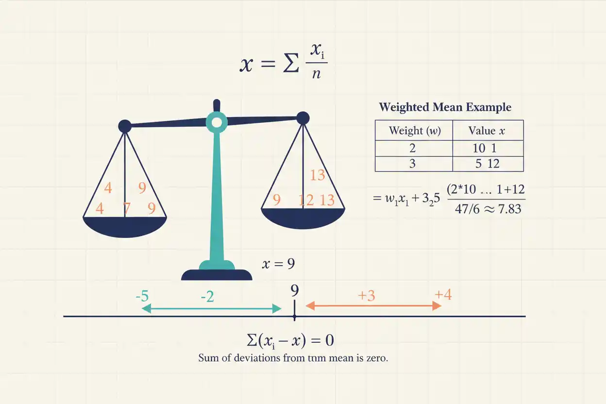
The arithmetic mean is a measure of central tendency found by adding numerical values and dividing their total by the number of values, making it the most familiar mathematical definition of an average. For a sample, the arithmetic mean is written x̄ = Σxᵢ/n, while a finite population mean is commonly written μ = Σxᵢ/N, with the symbols distinguishing a statistic calculated from observed sample data from a parameter describing an entire population. The arithmetic mean incorporates every numerical observation, which gives it powerful mathematical properties and makes it central to variance, standard deviation, regression, sampling distributions, confidence intervals, and many other statistical methods, but the same dependence on every value also makes it sensitive to extreme observations and skewed distributions. It can be extended naturally to weighted observations, frequency tables, grouped data, and combined groups, provided the weights and denominators accurately represent the quantities being averaged. A useful interpretation is that the arithmetic mean is the numerical balance point of the data: observations above it have positive deviations, observations below it have negative deviations, and those signed deviations sum exactly to zero.
The arithmetic mean is a core measure within descriptive statistics and the broader Statistics & Probability framework. Although its formula is simple, correct use requires understanding what is being averaged, how observations are weighted, whether the distribution is distorted by unusually large or small values, and whether the mean is being used merely to describe observed data or to estimate an unknown population quantity.
What Is the Arithmetic Mean?
The arithmetic mean is calculated by summing all numerical observations and dividing by their count.
For values:
x₁, x₂, …, xₙ
the sample arithmetic mean is:
x̄ = (x₁ + x₂ + … + xₙ)/n
Using summation notation:
x̄ = Σxᵢ/n
Suppose the observations are:
4, 6, 8, 10, 12
Their total is:
4 + 6 + 8 + 10 + 12 = 40
and there are:
n = 5
observations.
Therefore:
x̄ = 40/5
x̄ = 8
The arithmetic mean is:
8
which lies at the center of this symmetric data set.
Arithmetic Mean Formula
For a sample:
x̄ = Σxᵢ/n
where:
- x̄ = sample arithmetic mean
- xᵢ = individual sample observation
- n = number of observations
- Σ = sum across the observations
For a finite population:
μ = Σxᵢ/N
where:
- μ = population arithmetic mean
- N = population size
The arithmetic operation is structurally the same in both cases. The notation changes because the statistical role changes.
A sample mean is calculated from a subset of data and can estimate an unknown population mean, whereas a population mean describes the complete population itself.
Arithmetic Mean Example
Consider:
7, 9, 12, 13, 14
First add the observations:
7 + 9 + 12 + 13 + 14 = 55
Count them:
n = 5
Then divide:
x̄ = 55/5
x̄ = 11
Therefore, the arithmetic mean is:
11
Notice that 11 does not need to appear among the original observations. A mean represents the arithmetic balance of the values rather than necessarily identifying one actual observation.
Why Is It Called the Arithmetic Mean?
The term distinguishes this mean from other mathematical averages such as:
- geometric mean,
- harmonic mean,
- quadratic mean.
The arithmetic mean uses ordinary addition:
Σxᵢ
followed by division by the number of observations.
For example, the arithmetic mean of:
2 and 8
is:
(2 + 8)/2
= 5
The geometric mean would instead be:
√(2 × 8)
= 4
Different means answer different mathematical questions.
The arithmetic mean is the natural average for additive quantities.
The Arithmetic Mean as a Balance Point
One of the most important properties of the arithmetic mean is:
Σ(xᵢ − x̄) = 0
In words, the signed deviations from the mean sum to zero.
Consider:
2, 4, 6, 8, 10
with:
x̄ = 6
The deviations are:
−4, −2, 0, 2, 4
Add them:
−4 − 2 + 0 + 2 + 4 = 0
The negative deviations below the mean exactly balance the positive deviations above it.
This property is why the arithmetic mean can be interpreted as a numerical equilibrium point.
Why Deviations From the Mean Sum to Zero
Start with:
Σ(xᵢ − x̄)
Distribute the summation:
Σxᵢ − Σx̄
Because x̄ is constant across all n observations:
Σx̄ = nx̄
and by definition:
nx̄ = Σxᵢ
Therefore:
Σ(xᵢ − x̄) = Σxᵢ − Σxᵢ
= 0
This identity is exact, apart from any numerical rounding used in practical calculations.
It also explains why ordinary signed deviations cannot be averaged directly to measure dispersion: their average is always zero around the arithmetic mean.
Population Arithmetic Mean
If every member of a finite population is observed, the population mean is:
μ = Σxᵢ/N
Suppose the entire population is:
3, 5, 7, 9
Then:
N = 4
and:
μ = (3 + 5 + 7 + 9)/4
μ = 24/4
μ = 6
Since all four population values are known, 6 is the actual mean of that defined finite population rather than an estimate based on a sample.
Sample Arithmetic Mean
Suppose:
3, 5, 7, 9
are instead four randomly selected observations from a much larger population.
Then:
n = 4
and:
x̄ = 6
The arithmetic calculation is unchanged, but the result now has a different statistical interpretation.
The sample mean:
x̄ = 6
is one possible estimate of the unknown population mean:
μ.
Another random sample could produce a different x̄ because different observations would be selected.
Mean vs Sum
The sum and arithmetic mean contain related but different information.
Suppose:
5, 10, 15
The sum is:
30
The mean is:
30/3 = 10
If every value is duplicated:
5, 10, 15, 5, 10, 15
the sum becomes:
60
but the mean remains:
60/6 = 10
The sum grows with the number of observations, whereas the arithmetic mean describes average magnitude independent of how many exact copies of the entire data set are included.
Mean With Negative Numbers
Negative observations are handled in exactly the same way.
Consider:
−8, −4, 2, 6
Their sum is:
−8 − 4 + 2 + 6
= −4
Therefore:
x̄ = −4/4
= −1
The arithmetic mean is:
−1
A negative mean simply indicates that the numerical balance point lies below zero.
There is no requirement that observations or their mean be positive.
Mean With Decimals
The arithmetic mean can also be calculated from decimal values.
Suppose:
2.4, 3.1, 4.7, 5.8
Their total is:
16.0
and:
n = 4
Therefore:
x̄ = 16/4
= 4
The result can be an integer even when none of the inputs are integers.
Likewise, integer observations can produce a noninteger mean.
Arithmetic Mean of Percentages
Percentages can sometimes be averaged arithmetically, but only when each percentage should receive equal weight.
Suppose three equally weighted observations are:
60%, 70%, 80%
Then:
Mean percentage = (60 + 70 + 80)/3
= 70%
However, if the percentages come from groups of different sizes, the ordinary arithmetic mean can be misleading.
For example, averaging:
90% from 10 observations
and:
50% from 1,000 observations
as:
(90% + 50%)/2 = 70%
gives the two groups equal influence despite dramatically different denominators.
A weighted calculation is more appropriate when the underlying group sizes differ.
Weighted Arithmetic Mean
A weighted arithmetic mean allows observations to contribute unequally.
The formula is:
x̄w = Σwᵢxᵢ / Σwᵢ
where:
- xᵢ = value
- wᵢ = weight attached to that value
Suppose:
x₁ = 70 with weight 1
x₂ = 80 with weight 2
x₃ = 90 with weight 3
The weighted total is:
1(70) + 2(80) + 3(90)
= 70 + 160 + 270
= 500
Total weight is:
1 + 2 + 3 = 6
Therefore:
x̄w = 500/6
≈ 83.33
The largest weight gives the value 90 the greatest influence.
Weighted Mean vs Ordinary Mean
Using the same values:
70, 80, 90
the ordinary arithmetic mean is:
(70 + 80 + 90)/3
= 80
The weighted arithmetic mean was:
83.33
because 90 received three times as much weight as 70.
Neither result is universally more correct.
The appropriate calculation depends on whether the observations genuinely have equal or unequal statistical importance.
Weights should represent something meaningful, such as frequency, credit hours, exposure, or sampling structure.
Grade Weighted Mean Example
Suppose course components are:
| Component | Score | Weight |
|---|---|---|
| Assignment | 80 | 20% |
| Midterm | 70 | 30% |
| Final | 90 | 50% |
Convert the percentages to decimal weights:
0.20, 0.30, 0.50
Then:
Weighted mean = 80(0.20) + 70(0.30) + 90(0.50)
= 16 + 21 + 45
= 82
Because the weights sum to:
1
there is no additional division required.
The weighted course average is:
82
Arithmetic Mean From a Frequency Table
When values repeat, a frequency table can simplify the calculation.
Suppose:
| Value x | Frequency f |
|---|---|
| 1 | 2 |
| 2 | 3 |
| 3 | 4 |
| 4 | 1 |
The total frequency is:
n = 2 + 3 + 4 + 1
n = 10
Calculate:
Σfx = 1(2) + 2(3) + 3(4) + 4(1)
= 2 + 6 + 12 + 4
= 24
Therefore:
x̄ = Σfx/Σf
= 24/10
= 2.4
This is equivalent to expanding all ten observations individually and calculating their ordinary mean.
Mean From Relative Frequencies
If relative frequencies sum to one, the arithmetic mean can be calculated as:
x̄ = Σrᵢxᵢ
where rᵢ is the relative frequency.
Using the previous table:
Value 1 → relative frequency 0.2
Value 2 → 0.3
Value 3 → 0.4
Value 4 → 0.1
Then:
x̄ = 1(0.2) + 2(0.3) + 3(0.4) + 4(0.1)
= 0.2 + 0.6 + 1.2 + 0.4
= 2.4
The result matches the frequency-based calculation.
Arithmetic Mean From Grouped Data
When raw observations are unavailable and only class intervals are known, an approximate mean can be calculated using class midpoints.
Suppose:
| Interval | Frequency |
|---|---|
| 0–10 | 5 |
| 10–20 | 8 |
| 20–30 | 7 |
Class midpoints are:
5, 15, 25
The approximate grouped mean is:
x̄ ≈ Σfm / Σf
where m is the midpoint.
Calculate:
Σfm = 5(5) + 8(15) + 7(25)
= 25 + 120 + 175
= 320
Total frequency:
n = 20
Therefore:
x̄ ≈ 320/20
x̄ ≈ 16
This is an approximation because the actual observations within each interval are unknown.
Why the Grouped Mean Is Approximate
The midpoint method acts as though every observation in a class lies exactly at the class midpoint.
For the interval:
10–20
it treats all observations as:
In reality, values could be concentrated near 10, near 20, or distributed unevenly throughout the interval.
If the within-class distribution is reasonably balanced and the intervals are sufficiently narrow, the midpoint approximation can be useful.
If intervals are wide or highly uneven internally, the approximation can differ noticeably from the mean of the original raw data.
Arithmetic Mean From Cumulative Frequency
A cumulative frequency table records running totals rather than individual frequencies, so the ordinary frequencies must generally be recovered before calculating the mean.
Suppose cumulative frequencies are:
| Value | Cumulative Frequency |
|---|---|
| 1 | 3 |
| 2 | 8 |
| 3 | 12 |
| 4 | 15 |
Then ordinary frequencies are:
f₁ = 3
f₂ = 8 − 3 = 5
f₃ = 12 − 8 = 4
f₄ = 15 − 12 = 3
Once those frequencies are recovered, use:
x̄ = Σfx/Σf
to calculate the arithmetic mean.
Combined Arithmetic Mean
If separate groups have known means and sample sizes, the overall mean can be calculated without reconstructing every individual observation.
For two groups:
Combined mean = (n₁x̄₁ + n₂x̄₂)/(n₁ + n₂)
Suppose:
Group A: n₁ = 20, x̄₁ = 70
Group B: n₂ = 30, x̄₂ = 80
Then:
Combined mean = [20(70) + 30(80)]/50
= (1400 + 2400)/50
= 3800/50
= 76
The overall mean is:
76
not:
75
because the group with mean 80 contains more observations and therefore receives more weight.
Why Averaging Group Means Can Be Wrong
Using the previous groups:
Mean A = 70
Mean B = 80
A simple average of the two group means gives:
(70 + 80)/2
= 75
But this treats the groups as equally large.
The correct combined mean is:
76
because one group contains:
30 observations
while the other contains:
A simple arithmetic mean of subgroup means is correct only when the groups have equal size or when equal weighting of the groups is intentionally desired.
Mean After Adding a Constant
Suppose every observation is increased by the same constant c:
yᵢ = xᵢ + c
Then:
ȳ = x̄ + c
For example, start with:
2, 4, 6
whose mean is:
Add:
10
to every value:
12, 14, 16
The new mean is:
14
which equals:
4 + 10.
Adding a constant shifts the entire distribution and its arithmetic mean by exactly the same amount.
Mean After Multiplication
If every observation is multiplied by a constant a:
yᵢ = axᵢ
then:
ȳ = ax̄
Suppose:
2, 4, 6
have mean:
Multiply every value by:
5
to obtain:
10, 20, 30.
The new mean is:
20
which equals:
5(4).
Thus, multiplication rescales the arithmetic mean in the same way it rescales the observations.
Mean Under a Linear Transformation
Combining both properties:
Y = aX + b
implies:
Mean(Y) = aMean(X) + b
For a population:
μY = aμX + b
For a sample:
ȳ = ax̄ + b
This relationship is useful for unit conversions.
For example, if a temperature variable is transformed through a linear scale conversion, its arithmetic mean can be converted using the same transformation without recalculating every observation individually.
Effect of Changing One Observation
Suppose a sample contains n observations with mean x̄.
If one observation increases by:
d
while every other value remains unchanged, the total sum increases by d.
Therefore, the new mean becomes:
New mean = x̄ + d/n
For example, if:
n = 10
and one observation increases by:
20
then the mean increases by:
20/10
= 2
This relationship helps explain how the influence of one observation on the mean decreases as sample size becomes larger.
Effect of Adding One New Observation
Suppose n observations have mean:
x̄old
and one new value:
xnew
is added.
The old total is:
n x̄old
The new mean is:
x̄new = (n x̄old + xnew)/(n + 1)
Suppose:
n = 4
x̄old = 10
and:
xnew = 20
Then:
x̄new = [4(10) + 20]/5
= 60/5
= 12
This formula allows a mean to be updated without storing or re-summing all previous observations.
Updating a Mean With Multiple New Observations
Suppose an existing group has:
n₁ observations
with mean:
x̄₁
and a new group has:
n₂ observations
with mean:
x̄₂.
The combined mean is:
x̄combined = (n₁x̄₁ + n₂x̄₂)/(n₁+n₂)
This is mathematically the same weighted-mean principle used when combining groups.
The number of observations acts as the weight assigned to each subgroup mean.
This relationship is useful when data arrive in batches.
Arithmetic Mean and Missing Values
Missing observations should not automatically be treated as zero.
Suppose the recorded data are:
10, 20, missing, 30
If the missing observation is excluded and the mean is calculated over available values:
x̄ = (10 + 20 + 30)/3
= 20
If the missing value is incorrectly entered as zero:
x̄ = (10 + 20 + 0 + 30)/4
= 15
The result changes materially.
Missing-data handling is therefore a substantive statistical decision, not merely a detail of the mean formula.
Arithmetic Mean and Outliers
The arithmetic mean is sensitive to extreme observations because every value enters the total directly.
Consider:
10, 11, 12, 13, 14
The mean is:
12
Now replace:
14
with:
100
The new mean becomes:
(10 + 11 + 12 + 13 + 100)/5
= 146/5
= 29.2
Four of five observations remain between 10 and 13, yet the mean moves from 12 to 29.2.
This illustrates why the mean can provide a misleading impression of a “typical” value in highly skewed or contaminated data.
Arithmetic Mean vs Median
The arithmetic mean uses every numerical magnitude.
The median depends primarily on ordered position.
Consider:
2, 3, 4, 5, 100
The mean is:
114/5
= 22.8
The median is:
4
The median remains near the central cluster, while the mean is pulled strongly toward the large upper-tail value.
For symmetric distributions without problematic extremes, mean and median can be similar. For strongly skewed data, reporting both can reveal important distribution structure.
Arithmetic Mean vs Five-Number Summary
A mean compresses all numerical observations into one arithmetic balance point, whereas a five-number summary describes a distribution through:
Minimum
Q₁
Median
Q₃
Maximum
The five-number summary can reveal asymmetry and tail spread that the mean alone cannot show.
Two data sets can have the same arithmetic mean while possessing very different quartiles and extremes.
These summaries are therefore complementary rather than substitutes for one another.
Arithmetic Mean and Box Plots
A standard box plot is based primarily on quartiles and the median rather than the arithmetic mean.
Its box typically spans:
Q₁ to Q₃
with the median marked inside.
Some customized box plots also display the mean as a separate symbol, but it is not part of the basic five-number structure.
Comparing the plotted median with an added mean marker can provide useful descriptive clues about asymmetry, particularly when a long tail pulls the arithmetic mean away from the center of the box.
Mean and Skewness
In a strongly right-skewed distribution, unusually large values often pull the arithmetic mean above the median.
In a left-skewed distribution, unusually small values often pull the mean below the median.
For example:
2, 3, 4, 5, 30
has:
Mean = 8.8
Median = 4
The large upper-tail observation raises the mean substantially.
However, mean-median ordering is not a universal definition of skewness. Distribution shape should be assessed from the data as a whole, ideally using graphs and positional summaries.
Arithmetic Mean and Variance
Variance is calculated from squared deviations around the arithmetic mean.
For a population:
σ² = Σ(xᵢ − μ)²/N
For a conventional sample variance:
s² = Σ(xᵢ − x̄)²/(n − 1)
Thus, the arithmetic mean provides the center around which variance measures dispersion.
This relationship is not arbitrary. The arithmetic mean has a unique least-squares property that makes the total squared deviations smallest when they are measured from the mean.
Least-Squares Property of the Arithmetic Mean
Consider choosing any constant c and calculating:
Σ(xᵢ − c)²
The value of c that minimizes this squared-error total is:
c = x̄
for sample data.
Therefore:
Σ(xᵢ − x̄)² ≤ Σ(xᵢ − c)²
for every other constant c.
This least-squares property connects the arithmetic mean directly with variance and regression.
It explains why squared-error statistical methods naturally produce arithmetic means as fitted centers.
Arithmetic Mean and Expected Value
In probability theory, the expected value of a random variable is the population analogue of a probability-weighted arithmetic mean.
For a discrete random variable:
E(X) = ΣxP(X=x)
Suppose X can equal:
0, 1, 2
with probabilities:
0.25, 0.50, 0.25
Then:
E(X) = 0(0.25) + 1(0.50) + 2(0.25)
= 1
The expected value is the probability-weighted arithmetic center of the distribution.
It need not correspond to an outcome that occurs in every trial.
Mean of a Sum
Expected values and arithmetic means have an important additive property.
For random variables X and Y:
E(X + Y) = E(X) + E(Y)
regardless of whether X and Y are independent, provided the required expectations exist.
For finite data, a related arithmetic identity means that if two variables are added observation by observation, the mean of the resulting sums equals the sum of their respective means:
Mean(X + Y) = Mean(X) + Mean(Y)
This linearity is one reason the arithmetic mean is mathematically convenient.
Mean of a Difference
Likewise:
E(X − Y) = E(X) − E(Y)
and for paired finite observations:
Mean(X − Y) = Mean(X) − Mean(Y)
when the means are calculated over corresponding pairs.
This property is especially useful when studying change scores.
If:
Mean before = 50
and:
Mean after = 55
then the mean of the paired differences:
After − Before
is:
5
provided the same complete set of paired units is used in both calculations.
Arithmetic Mean and Confidence Intervals
When the arithmetic mean is calculated from a sample, it can serve as a point estimate of an unknown population mean.
A confidence interval adds information about the sampling uncertainty around that estimate.
A common interval structure is:
x̄ ± Critical value × Standard error
For example, if:
x̄ = 100
SE = 2
and an appropriate 95% critical value is approximately:
1.96
the interval is:
100 ± 1.96(2)
= 100 ± 3.92
or:
(96.08, 103.92)
The arithmetic mean provides the center of the interval, while the standard error and critical value determine its width.
Arithmetic Mean and Sample Size
A larger sample does not automatically change the population mean being estimated, but it generally makes the sample mean more stable under independent representative sampling.
If observations have population standard deviation σ:
SE(X̄) = σ/√n
Therefore, increasing n narrows the sampling distribution of x̄.
For example, if:
σ = 20
then at:
n = 25
the standard error is:
20/5 = 4
while at:
n = 100
it is:
20/10 = 2
The raw observations remain equally variable; the arithmetic mean becomes more precise as an estimator.
Arithmetic Mean and Coefficient of Variation
The coefficient of variation expresses standard deviation relative to the arithmetic mean:
CV = s/x̄
for a common sample form.
Suppose:
x̄ = 50
and:
s = 5
Then:
CV = 5/50
= 0.10
or:
10%
The mean acts as the reference level against which variability is scaled.
Because of this denominator, the coefficient of variation requires caution when the arithmetic mean is close to zero or when the measurement scale does not have a meaningful absolute zero.
Arithmetic Mean of Ratios
A common source of error is averaging ratios without considering their denominators.
Suppose one trip covers:
100 km in 1 hour
and another covers:
100 km in 2 hours.
The speeds are:
100 km/h
and:
50 km/h.
The simple arithmetic mean of the two speeds is:
75 km/h
but total distance is:
200 km
and total time is:
3 hours
so overall average speed is:
200/3
≈ 66.67 km/h.
The arithmetic mean of individual rates is correct only under appropriate weighting conditions.
For equal distances, the harmonic mean is often relevant for average speed.
Arithmetic Mean of Growth Rates
Arithmetic averaging can also be misleading for compounded growth.
Suppose an investment changes by:
+50%
in one period and:
−50%
in the next.
The arithmetic mean return is:
(50% − 50%)/2
= 0%
Yet an initial value of:
100
becomes:
150
and then:
The two-period compounded result is a loss, not zero growth.
When quantities compound multiplicatively, geometric averaging is often more appropriate than the arithmetic mean.
When the Arithmetic Mean Is Appropriate
The arithmetic mean is especially useful when:
- observations are numerical,
- addition is substantively meaningful,
- each observation should receive equal weight unless explicit weights are supplied,
- the arithmetic balance point is relevant,
- extreme values do not make the center misleading.
Examples include many measurements of:
height,
temperature changes,
test scores,
production quantities,
errors,
provided the measurement and distribution support mean-based interpretation.
It is also indispensable when later statistical procedures are mathematically defined around the mean.
When the Arithmetic Mean Can Be Misleading
The arithmetic mean can be a poor standalone summary when:
- the distribution is strongly skewed,
- a few extreme observations dominate the total,
- values belong to fundamentally different subgroups,
- the data are categorical labels,
- ratios require unequal weighting,
- growth compounds multiplicatively,
- missing values are handled incorrectly.
For example, an average income can be far above the income of a typical person in a highly right-skewed population.
In such cases, median, quantiles, subgroup summaries, or alternative means can provide essential context.
Arithmetic Mean for Categorical Data
An arithmetic mean generally should not be calculated for unordered categorical labels.
Suppose categories are coded:
Red = 1
Blue = 2
Green = 3
A numerical mean such as:
2.1
does not represent a meaningful “average color.”
The numerical codes are identifiers rather than measurements.
Frequency, proportion, and mode are more appropriate descriptive statistics for nominal categorical variables.
Arithmetic Mean for Ordinal Data
Ordinal categories have a natural order but not necessarily equal numerical spacing.
For example:
Poor
Fair
Good
Excellent
can be coded:
1, 2, 3, 4
but the distance between “Poor” and “Fair” is not necessarily psychologically or substantively equal to the distance between “Good” and “Excellent.”
An arithmetic mean of those codes can therefore impose an interval interpretation that the scale may not support.
Whether averaging ordinal scores is useful depends on the measurement model and analytical context.
Arithmetic Mean and Duplicated Observations
Duplicating every observation an equal number of times does not change the mean.
Suppose:
2, 4, 6
has mean:
Duplicate the entire set:
2, 4, 6, 2, 4, 6
The total becomes:
24
and n becomes:
6
so:
x̄ = 24/6
= 4
The mean remains unchanged because both the sum and observation count increase by the same factor.
Arithmetic Mean Must Lie Between Minimum and Maximum
For a nonempty set of ordinary real-valued observations with equal positive weights:
Minimum ≤ Mean ≤ Maximum
For example:
3, 8, 20
cannot have an arithmetic mean below 3 or above 20.
Indeed:
x̄ = 31/3
≈ 10.33
which lies within the observed range.
A calculated mean outside the minimum-maximum interval indicates an arithmetic or data-handling mistake unless unusual negative weighting or another nonstandard calculation is involved.
The Mean Need Not Be an Observed Value
Consider:
1, 2
The arithmetic mean is:
1.5
although neither observation equals 1.5.
Likewise, if a data set counts children per household, the mean could be:
1.8 children
even though no household literally contains 1.8 children.
The mean summarizes the distribution; it does not have to correspond to a physically attainable individual observation.
This distinction is important for discrete variables.
Mean and Subgroup Composition
An overall arithmetic mean can change because subgroup proportions change even if each subgroup’s own mean stays constant.
Suppose:
Group A mean = 50
Group B mean = 100
If the population initially contains equal numbers of A and B:
Overall mean = 75.
If later:
90%
of observations belong to A and:
10%
to B, the overall mean becomes:
0.9(50) + 0.1(100)
= 55.
Neither subgroup mean changed.
Only the composition changed.
Overall averages should therefore be interpreted alongside important subgroup structure.
Common Arithmetic Mean Mistakes
A common mistake is adding observations correctly but dividing by the wrong count. The denominator should represent the number of equally weighted observations or, for a weighted mean, the total appropriate weight.
Another error is averaging subgroup means without weighting them by subgroup size when the goal is an overall observation-level mean.
A third mistake is treating missing observations as zero even when zero is not their actual value.
Another frequent problem is applying the arithmetic mean to nominal categories whose numerical codes have no quantitative meaning.
Analysts may also average percentages, rates, or ratios that have different underlying denominators without applying the necessary weights.
Another mistake is using the arithmetic mean as the only description of highly skewed data, where a median or box plot can reveal important structure hidden by the average.
Finally, a sample mean should not be presented as though it were the exact population mean when the analysis is based on only a sample.
How to Calculate the Arithmetic Mean Step by Step
First identify the numerical observations and determine whether they should receive equal weight. Check missing values, inconsistent units, and duplicated records before calculating the total.
For an ordinary arithmetic mean, add all valid observations:
Total = Σxᵢ
Count them:
n
Then divide:
x̄ = Σxᵢ/n
For weighted observations, multiply each value by its weight, add the weighted values, and divide by the total weight:
x̄w = Σwᵢxᵢ/Σwᵢ
For a frequency table, frequencies serve as weights. For grouped intervals, use class midpoints only when an approximate grouped-data mean is acceptable.
Finally, interpret the result in the measurement context and examine whether skewness or extreme observations make the arithmetic mean insufficient as a standalone summary.
Full Worked Arithmetic Mean Example
Consider the sample:
6, 8, 9, 11, 13, 15, 22
There are:
n = 7
observations.
Add them:
6 + 8 + 9 + 11 + 13 + 15 + 22
= 84
Then:
x̄ = 84/7
= 12
Therefore:
Arithmetic mean = 12
Now calculate deviations:
−6, −4, −3, −1, 1, 3, 10
Their sum is:
−6 − 4 − 3 − 1 + 1 + 3 + 10
= 0
This confirms the balance-point property of the arithmetic mean.
The upper value of 22 contributes substantially to the total, so comparing the mean with the median can provide additional context.
Median Comparison for the Worked Example
The ordered data are:
6, 8, 9, 11, 13, 15, 22
The median is:
11
while the arithmetic mean is:
The mean is slightly higher because the upper value:
22
pulls the arithmetic balance point upward.
The difference is not extreme, but it illustrates how values far from the center affect the mean more directly than the median.
A five-number summary can provide additional information about the positions and tails of the distribution.
Full Weighted Mean Example
Suppose four values have the following weights:
| Value | Weight |
|---|---|
| 50 | 1 |
| 60 | 2 |
| 80 | 4 |
| 100 | 3 |
Calculate the weighted products:
50(1) = 50
60(2) = 120
80(4) = 320
100(3) = 300
Total weighted value:
50 + 120 + 320 + 300 = 790
Total weight:
1 + 2 + 4 + 3 = 10
Therefore:
x̄w = 790/10
= 79
The weighted arithmetic mean is:
79
whereas the unweighted mean of the four distinct values would be:
(50 + 60 + 80 + 100)/4
= 72.5
The difference demonstrates the importance of correctly representing the weights.
Full Frequency-Table Example
Suppose scores occur with these frequencies:
| Score | Frequency |
|---|---|
| 10 | 2 |
| 20 | 5 |
| 30 | 2 |
| 40 | 1 |
Calculate:
Σf = 2 + 5 + 2 + 1
= 10
Then:
Σfx = 10(2) + 20(5) + 30(2) + 40(1)
= 20 + 100 + 60 + 40
= 220
Therefore:
x̄ = 220/10
= 22
The arithmetic mean is:
22
even though 22 does not appear as an observed score.
How to Report the Arithmetic Mean
A clear report should identify the arithmetic mean, the units, and the amount of data supporting it.
For example:
“The sample contained n = 120 observations with an arithmetic mean of 52.4 units.”
Because a mean alone gives no information about spread, it is often helpful to report a dispersion measure:
“Mean = 52.4, SD = 8.1.”
If the distribution is visibly skewed or contains influential extremes, add robust positional information or a graphical summary rather than relying on the mean alone.
If the sample mean is being used for population inference, distinguish the descriptive estimate from the uncertainty represented by its standard error or confidence interval.
Frequently Asked Questions About the Arithmetic Mean
What is the arithmetic mean?
The arithmetic mean is the sum of numerical observations divided by the number of observations.
What is the sample arithmetic mean formula?
x̄ = Σxᵢ/n
What is the population arithmetic mean formula?
μ = Σxᵢ/N
Is arithmetic mean the same as average?
In ordinary numerical usage, “average” often refers to the arithmetic mean, although the word average can also be used more broadly for other measures of center.
How do you calculate an arithmetic mean?
Add all valid values and divide the total by their count.
Can an arithmetic mean be a decimal?
Yes.
Can the arithmetic mean be negative?
Yes.
Can the arithmetic mean be zero?
Yes, when the positive and negative values balance arithmetically around zero.
Can the arithmetic mean be a value not present in the data?
Yes. The mean is a balance point and need not correspond to an actual observation.
Does the arithmetic mean always lie between the minimum and maximum?
Yes, for ordinary equally weighted real-valued data and positive conventional weights.
Why do deviations from the mean sum to zero?
Because:
Σ(xᵢ − x̄) = Σxᵢ − nx̄ = 0
by the definition of x̄.
Is the arithmetic mean affected by outliers?
Yes. Extreme observations can strongly influence it.
Is the arithmetic mean robust?
No. The median and rank-based summaries are generally more resistant to extremes.
What is the difference between mean and median?
The mean uses every numerical value, while the median is determined primarily by ordered position.
When is the median preferable?
It can provide a more representative central summary when data are strongly skewed or heavily affected by extreme observations.
What is a weighted arithmetic mean?
It gives observations unequal influence:
x̄w = Σwᵢxᵢ/Σwᵢ
When should a weighted mean be used?
When observations genuinely have different frequencies, exposures, importance, credits, or other meaningful weights.
How is the mean calculated from a frequency table?
x̄ = Σfx/Σf
where f is frequency.
How is the arithmetic mean calculated from grouped data?
A common approximation is:
x̄ ≈ Σfm/Σf
where m is the class midpoint.
Is a grouped mean exact?
Not usually. It is approximate because individual observations inside each class are unknown.
How do you combine two group means?
x̄combined = (n₁x̄₁ + n₂x̄₂)/(n₁+n₂)
Can you simply average two group means?
Only when equal group weighting is intended; for an observation-level overall mean, subgroup sizes must generally be used as weights.
What happens to the mean if every value increases by c?
The mean also increases by c.
What happens if every value is multiplied by a?
The mean is multiplied by a.
What is the mean after a linear transformation Y = aX + b?
Mean(Y) = aMean(X) + b
What happens if one observation increases by d?
For a fixed sample of n observations, the mean increases by:
d/n
How do you update a mean after adding one new value?
x̄new = (n x̄old + xnew)/(n+1)
Is the arithmetic mean appropriate for percentages?
It can be when percentages are equally weighted. Different denominators often require a weighted calculation.
Is arithmetic mean appropriate for average speed?
Sometimes, but not always. When equal distances are traveled at different speeds, a harmonic rather than arithmetic mean can be relevant.
Is arithmetic mean appropriate for compound growth?
Not usually for multi-period compounded growth. A geometric mean often better represents multiplicative growth factors.
Can you calculate an arithmetic mean for categories?
Not meaningfully for nominal categories whose numerical labels are arbitrary.
How is arithmetic mean related to variance?
Variance measures squared deviations around the arithmetic mean.
Why is the arithmetic mean important in least squares?
It is the constant that minimizes the sum of squared deviations from the observations.
How is arithmetic mean related to expected value?
Expected value is a probability-weighted population mean for a random variable.
How is arithmetic mean used in confidence intervals?
The sample mean commonly serves as the point estimate at the center of a confidence interval for the population mean.
Does a larger sample change the arithmetic mean formula?
No. The formula remains:
x̄ = Σxᵢ/n
but larger representative samples generally make x̄ more stable as an estimator of μ.
Can two data sets have the same arithmetic mean but very different distributions?
Yes. They can differ greatly in variance, quartiles, skewness, tails, or subgroup structure.
What is the most important rule when using the arithmetic mean?
Use it when arithmetic averaging matches the measurement and weighting structure, and interpret it together with spread and distribution shape whenever skewness, extreme values, or subgroup differences could make one average incomplete.




