

Coefficient Of Variation: Definition, Formula & Example

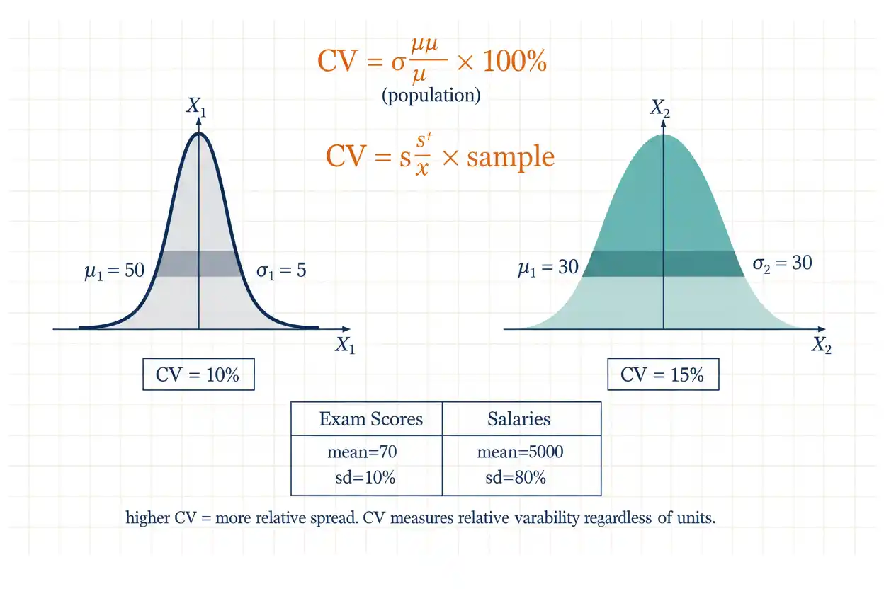
The coefficient of variation is a dimensionless measure of relative variability that compares a standard deviation with the corresponding arithmetic mean, making it useful when the objective is to compare dispersion across data sets whose typical magnitudes differ substantially. Instead of reporting variability only in the original measurement units, the coefficient of variation expresses spread as a fraction or percentage of the mean, so a standard deviation of 10 can represent relatively little variation when the mean is 1,000 but extremely large variation when the mean is 12. For a population with positive mean μ and standard deviation σ, the coefficient of variation is commonly calculated as CV = σ/μ, while sample data usually use CV = s/x̄, with multiplication by 100 converting the ratio to a percentage. This scale-free property makes the coefficient of variation particularly useful for suitable positive ratio-scale measurements, including production quantities, physical measurements, concentrations, durations, and other variables for which ratios such as “twice as large” have meaningful interpretations. However, the measure becomes unstable when the mean is close to zero, can become difficult or misleading when the mean is negative, and is generally inappropriate for interval scales whose zero point is arbitrary because adding a constant changes the coefficient of variation even though the underlying physical spread has not changed.
The coefficient of variation belongs to the broader framework of descriptive statistics within Statistics & Probability. It complements absolute measures of spread by answering a specifically relative question: how large is the standard deviation compared with the arithmetic level around which the observations are centered?
What Is the Coefficient of Variation?
The coefficient of variation compares the size of standard deviation with the size of the mean.
For a population:
CV = σ/μ
When expressed as a percentage:
CV% = (σ/μ) × 100%
For a sample:
CV = s/x̄
or:
CV% = (s/x̄) × 100%
where:
- CV = coefficient of variation
- σ = population standard deviation
- μ = population mean
- s = sample standard deviation
- x̄ = sample arithmetic mean
The calculation therefore combines a measure of spread with a measure of center.
A CV of:
0.15
is commonly reported as:
15%
meaning the standard deviation is 15% of the mean.
Coefficient of Variation Formula
For population data:
CV = σ/μ
and:
CV% = 100(σ/μ)
For sample data:
CV = s/x̄
and:
CV% = 100(s/x̄)
The percentage and decimal forms contain the same information.
For example:
CV = 0.08
is equivalent to:
CV = 8%
The percentage version is often easier to communicate, while the decimal version can be more convenient inside calculations.
Simple Coefficient of Variation Example
Suppose a sample has:
x̄ = 50
and:
s = 5
Then:
CV = 5/50
= 0.10
Expressed as a percentage:
CV% = 0.10 × 100
= 10%
The sample standard deviation is therefore equal to:
10%
of the sample mean.
This indicates considerably lower relative variability than a sample with the same mean and:
s = 20
which would have:
CV = 40%.
Why Use the Coefficient of Variation?
Standard deviation measures absolute spread.
The coefficient of variation measures relative spread.
Consider two data sets:
A: Mean = 50, SD = 5
B: Mean = 500, SD = 20
Data set B has the larger standard deviation:
20 > 5
so it has greater absolute dispersion.
However:
CV_A = 5/50 = 0.10 = 10%
while:
CV_B = 20/500 = 0.04 = 4%
Relative to their respective means, A is more variable.
That is the central purpose of the coefficient of variation.
Absolute vs Relative Variability
Suppose two production processes manufacture components at very different scales.
Process A has:
Mean = 10 units
SD = 2 units
Process B has:
Mean = 1,000 units
SD = 50 units
Absolute variability favors Process A:
2 < 50
but relative variability tells a different story.
For A:
CV = 2/10
= 20%
For B:
CV = 50/1000
= 5%
Process B varies more in raw units but is much more consistent relative to its average level.
Both comparisons are mathematically valid because they answer different questions.
Population Coefficient of Variation
When the complete population is known, use:
CV = σ/μ
Suppose a population is:
40, 50, 60, 70, 80
Its population mean is:
μ = 60
The deviations are:
−20, −10, 0, 10, 20
Squared deviations are:
400, 100, 0, 100, 400
Their sum is:
1,000
Population variance is:
σ² = 1000/5
= 200
Therefore:
σ = √200
≈ 14.142
The population coefficient of variation is:
CV = 14.142/60
≈ 0.2357
or:
CV ≈ 23.57%
Sample Coefficient of Variation
Suppose the same observations:
40, 50, 60, 70, 80
are treated as a sample rather than the complete population.
The mean remains:
x̄ = 60
but sample variance is:
s² = 1000/(5 − 1)
= 250
Therefore:
s = √250
≈ 15.811
The sample coefficient of variation becomes:
CV = 15.811/60
≈ 0.2635
or:
26.35%
The difference arises because the sample standard deviation uses the n − 1 denominator.
Coefficient of Variation Step-by-Step Example
Consider the sample:
50, 55, 60, 65, 70
Step 1: Calculate the Mean
x̄ = (50 + 55 + 60 + 65 + 70)/5
x̄ = 300/5
x̄ = 60
Step 2: Calculate the Sample Standard Deviation
The deviations are:
−10, −5, 0, 5, 10
Squared deviations are:
100, 25, 0, 25, 100
Their sum is:
250
Sample variance:
s² = 250/(5 − 1)
= 62.5
Therefore:
s = √62.5
≈ 7.906
Step 3: Calculate the Coefficient of Variation
CV = 7.906/60
≈ 0.1318
Therefore:
CV ≈ 13.18%
The sample standard deviation is approximately 13.18% of the sample mean.
Interpreting a Coefficient of Variation
A coefficient of variation is usually interpreted comparatively rather than through a universal classification system.
For example:
CV = 5%
means standard deviation equals about 5% of the mean.
CV = 25%
means standard deviation equals about one quarter of the mean.
CV = 100%
means standard deviation equals the mean in magnitude.
A higher positive CV generally indicates greater relative dispersion when the compared variables are suitable for CV analysis.
A lower positive CV indicates greater relative consistency.
However, there is no universal statistical rule that labels every CV below a specific percentage as “good” or every larger value as “bad.” The acceptable amount of relative variability depends on the subject.
Is a Lower Coefficient of Variation Better?
A lower coefficient of variation means lower variability relative to the mean, but whether that is desirable depends on the problem.
For a manufacturing process where consistency is important:
lower CV
may be preferable.
For a naturally heterogeneous biological population, high relative variability may be an expected and meaningful feature rather than a defect.
For investment returns, interpreting CV can become especially problematic when the mean return is near zero or negative.
Thus:
lower CV = lower relative spread
is mathematically meaningful in suitable contexts, while:
lower CV = universally better
is not.
Why the Coefficient of Variation Is Dimensionless
Standard deviation and mean use the same measurement unit.
If both are measured in kilograms:
CV = kilograms/kilograms
so the units cancel.
If both are measured in meters:
CV = meters/meters
and again the units cancel.
Therefore, CV is dimensionless.
This is what allows relative variability to be compared across measurements with different numerical scales and, under appropriate conditions, even across different physical units.
Coefficient of Variation and Unit Conversion
Suppose a distance variable has:
Mean = 2 meters
SD = 0.10 meter
Then:
CV = 0.10/2
= 0.05
= 5%
Convert the same measurements to centimeters.
The mean becomes:
200 cm
and standard deviation becomes:
10 cm
Then:
CV = 10/200
= 0.05
= 5%
The coefficient of variation remains unchanged because both mean and standard deviation are multiplied by the same positive scaling factor.
Proof of Scale Invariance
Suppose:
Y = aX
for:
a > 0.
Then:
μY = aμX
and:
σY = aσX
Therefore:
CV_Y = σY/μY
= aσX/(aμX)
= σX/μX
Thus:
CV_Y = CV_X
The coefficient of variation is invariant to positive multiplicative rescaling.
This property is what makes it appropriate for comparing the same ratio-scale quantity measured in different units.
Adding a Constant Changes the CV
Now suppose:
Y = X + b
Then:
μY = μX + b
while:
σY = σX
because adding a constant does not change standard deviation.
Therefore:
CV_Y = σX/(μX + b)
which is generally not equal to:
σX/μX.
The coefficient of variation therefore changes when the zero point of the measurement scale changes.
This fact explains why CV should normally be used with ratio-scale variables whose zero has substantive meaning.
Why Ratio Scales Matter
A ratio scale has a meaningful absolute zero and supports statements such as:
20 kg is twice 10 kg.
Examples can include:
- mass,
- length,
- duration,
- concentration,
- positive production quantities.
For these variables, multiplying all measurements by a unit conversion factor preserves meaningful ratios.
The coefficient of variation therefore retains its interpretation.
An interval scale with an arbitrary zero does not have this property.
Why Celsius Is a Problem for CV
Consider temperatures:
20°C, 25°C, 30°C
The sample mean is:
25°C
and sample standard deviation is:
5°C
so:
CV = 5/25
= 20%
Now express the same physical temperatures in Kelvin:
293.15 K, 298.15 K, 303.15 K
The standard deviation remains:
5 K
but the mean becomes:
298.15 K
Therefore:
CV = 5/298.15
≈ 1.68%
The underlying temperature variation did not change physically, yet CV changed dramatically because Celsius and Kelvin differ by an additive constant.
This demonstrates why CV is inappropriate for scales with arbitrary zero points.
Coefficient of Variation vs Standard Deviation
Standard deviation reports spread in the original units.
Coefficient of variation reports spread relative to the mean.
Suppose:
| Data Set | Mean | SD | CV |
|---|---|---|---|
| A | 20 | 4 | 20% |
| B | 100 | 10 | 10% |
B has a larger absolute standard deviation:
10 > 4
but A has twice as much relative variability:
20% vs 10%.
Neither statistic replaces the other.
Standard deviation answers how much observations vary in raw units, while CV answers how large that variation is compared with the distribution’s arithmetic level.
Coefficient of Variation and Arithmetic Mean
The denominator of the coefficient of variation is the arithmetic mean, which means the behavior of CV depends strongly on that mean.
For sample data:
CV = s/x̄
If x̄ increases while s remains fixed, CV decreases.
If x̄ decreases toward zero while s remains fixed, CV grows rapidly.
This dependence is why CV can become unstable or meaningless for distributions whose means are near zero.
The mean is therefore not merely a scaling convenience; it is a critical part of whether CV has a sensible interpretation.
What Happens When the Mean Is Zero?
If:
μ = 0
then population CV would require:
CV = σ/0
which is undefined.
Similarly, if:
x̄ = 0
then the ordinary sample coefficient of variation:
s/x̄
is undefined.
Suppose data are:
−10, −5, 0, 5, 10
Their mean is:
0
but their standard deviation is positive.
The data clearly have variability, yet CV cannot express that variability relative to a zero mean.
An absolute dispersion measure should be used instead.
What Happens When the Mean Is Near Zero?
Suppose:
Mean = 0.1
and:
SD = 1
Then:
CV = 1/0.1
= 10
or:
1000%
A small change in the estimated mean can produce a dramatic change in CV.
For example, if the mean changes to:
0.05
while SD remains 1:
CV = 20
or:
2000%.
This numerical instability makes the coefficient of variation unreliable when the mean is close to zero.
What About Negative Means?
Suppose:
x̄ = −10
and:
s = 2
The direct formula gives:
CV = 2/(−10)
= −0.20
or:
−20%.
The negative sign comes from the denominator, not from negative variability, because standard deviation itself cannot be negative.
In many applications, this destroys the intended interpretation of CV as a positive relative-dispersion measure.
Some analysts use:
s/|x̄|
to force a positive value, but that is a modified convention that should be stated explicitly.
For ordinary CV comparison, positive ratio-scale data are the cleanest setting.
Can the Coefficient of Variation Exceed 100%?
Yes.
Suppose:
Mean = 20
SD = 30
Then:
CV = 30/20
= 1.5
or:
150%
There is no mathematical upper limit on CV when the positive mean can become small relative to standard deviation.
A CV greater than 100% means the standard deviation exceeds the mean.
That often indicates substantial relative dispersion, but it is not automatically an error.
Can the Coefficient of Variation Be Zero?
Yes.
If every observation has exactly the same positive value, then:
Standard deviation = 0
and therefore:
CV = 0/Mean
= 0.
For example:
20, 20, 20, 20
has:
Mean = 20
SD = 0
CV = 0%
A zero coefficient of variation means no observed variability relative to the mean.
Coefficient of Variation and Outliers
The coefficient of variation depends on both arithmetic mean and standard deviation, and both are sensitive to extreme observations.
Consider:
10, 11, 12, 13, 14
The mean is:
12
and sample standard deviation is approximately:
1.581
so:
CV ≈ 13.18%
Now replace 14 with:
Both the mean and standard deviation rise sharply.
The resulting CV can change dramatically, although its exact direction depends on how the extreme value affects the numerator relative to the denominator.
This makes CV non-robust to outliers.
Coefficient of Variation and Skewed Data
CV can be mathematically calculated for many skewed positive distributions, but it should be interpreted carefully because both mean and standard deviation are sensitive to long tails.
A strongly right-skewed distribution can have:
- a mean pulled toward large values;
- a standard deviation inflated by extreme observations.
The resulting CV may describe overall relative dispersion but still hide important distributional structure.
A box plot can provide complementary information about the median, quartiles, IQR, whiskers, and extreme observations without relying entirely on mean-based summaries.
Coefficient of Variation vs Five-Number Summary
The coefficient of variation compresses relative variability into one number.
A five-number summary describes a distribution through:
Minimum
Q₁
Median
Q₃
Maximum
These summaries answer different questions.
CV is particularly useful for comparing relative mean-centered spread.
The five-number summary is useful for understanding ordered position, range, central spread, and asymmetry.
Two distributions can have similar CVs but very different quartile structures or tail patterns.
Coefficient of Variation and Cumulative Frequency
A cumulative frequency table describes how observations accumulate across ordered values or intervals, whereas the coefficient of variation summarizes relative spread using only the mean and standard deviation.
Cumulative frequency preserves positional information that CV discards.
For example, two data sets can have:
the same mean
and:
the same standard deviation
and therefore the same CV, yet their cumulative frequency curves can have quite different shapes.
CV should therefore be understood as a compact dispersion measure rather than a complete distributional description.
Coefficient of Variation From Frequency Data
Suppose a frequency table is:
| Value x | Frequency f |
|---|---|
| 10 | 2 |
| 20 | 3 |
| 30 | 4 |
| 40 | 1 |
Total frequency is:
n = 10
Calculate the mean:
x̄ = Σfx/Σf
= [10(2) + 20(3) + 30(4) + 40(1)]/10
= (20 + 60 + 120 + 40)/10
= 240/10
= 24
The sample standard deviation can then be calculated using the weighted squared deviations and the appropriate sample denominator before applying:
CV = s/24.
Thus, frequency data do not change the definition; frequencies simply determine how often each value contributes.
Frequency-Table Sample CV Example
Continue with:
x̄ = 24
Calculate the weighted squared deviations:
For x = 10:
f(x − x̄)² = 2(10 − 24)²
= 2(196)
= 392
For x = 20:
3(20 − 24)² = 48
For x = 30:
4(30 − 24)² = 144
For x = 40:
1(40 − 24)² = 256
Total:
392 + 48 + 144 + 256
= 840
Sample variance:
s² = 840/(10 − 1)
≈ 93.333
Therefore:
s ≈ 9.661
and:
CV = 9.661/24
≈ 0.4025
or:
40.25%
The observations therefore have substantial variation relative to their mean.
Coefficient of Variation for Grouped Data
If only grouped intervals are available, an approximate CV can be calculated by first estimating the mean and standard deviation from class midpoints.
Suppose intervals have midpoints:
mᵢ
and frequencies:
fᵢ.
An approximate grouped mean is:
x̄ ≈ Σfᵢmᵢ/Σfᵢ
A grouped standard deviation can then be estimated from the same midpoint approximation.
Finally:
CV ≈ s_grouped/x̄_grouped
The result is approximate because every observation inside a class is represented by the class midpoint.
Wide intervals can therefore reduce accuracy.
Weighted Coefficient of Variation
When observations carry meaningful weights, the mean and standard deviation must be calculated using a weighting method consistent with what those weights represent.
A weighted descriptive mean is:
x̄w = Σwᵢxᵢ/Σwᵢ
A weighted dispersion measure can then be calculated around that weighted mean.
However, the correct denominator for a weighted sample variance is not universally:
Σw − 1.
Frequency weights, survey weights, probability weights, and analytic weights have different statistical meanings.
A weighted CV should therefore be based on a valid weighted mean and weighted standard deviation rather than applying ordinary sample formulas mechanically.
Comparing Two Coefficients of Variation
Suppose Laboratory A measures a quantity with:
Mean = 100
SD = 4
so:
CV_A = 4%
Laboratory B has:
Mean = 20
SD = 1.2
so:
CV_B = 6%
Although Laboratory B has the smaller absolute standard deviation:
1.2 < 4
it has the larger coefficient of variation:
6% > 4%.
Therefore, A has lower relative variability according to CV.
The comparison is meaningful only if the variables have compatible ratio-scale interpretations and represent comparable concepts.
Comparing Different Units
Suppose one measurement is expressed in grams and another in kilograms but both describe the same type of positive ratio-scale quantity.
Because CV is invariant to multiplicative unit changes, comparisons can remain meaningful.
For example:
Mean = 500 g
SD = 25 g
gives:
CV = 5%.
Expressing the same data as:
Mean = 0.5 kg
SD = 0.025 kg
still gives:
CV = 5%.
This unit invariance is one of CV’s principal advantages.
Comparing Different Variables
CV can sometimes compare relative variability across different ratio-scale variables, but the substantive interpretation still matters.
For example, one might compare relative variation in:
component mass
and:
production time
because both have meaningful positive zeros.
However, a numerically lower CV does not mean one variable is scientifically “better” than another.
The measure compares relative spread, not importance, accuracy, reliability, or desirability.
Those interpretations require additional context.
Coefficient of Variation and Measurement Precision
CV is often used to describe repeatability when measurement magnitude changes across conditions.
Suppose repeated measurements of a 10-unit reference have:
SD = 0.5
giving:
CV = 5%.
Measurements of a 100-unit reference have:
SD = 2
giving:
CV = 2%.
Although the second set has larger absolute variation, it is relatively more precise compared with its mean level.
This can make CV useful when measurement noise scales approximately with signal magnitude.
Precision Is Not Accuracy
A low CV indicates relatively low dispersion around the mean.
It does not establish that the mean is close to the true value.
Suppose a true reference is:
100
but a device repeatedly reports values near:
110
with:
Mean = 110
SD = 1
The CV is:
1/110
≈ 0.91%
which indicates high relative repeatability.
Yet the measurements are systematically about 10 units too high.
The process can therefore have a low CV while being inaccurate because of bias.
Coefficient of Variation and Reliability
CV is sometimes used informally as a consistency measure, but reliability has broader meanings depending on the discipline.
A low CV shows that observations are concentrated relative to their mean.
It does not prove:
- measurement validity;
- absence of systematic error;
- agreement between different instruments;
- temporal stability;
- causal consistency.
When those questions matter, additional statistical analyses are needed.
CV is a dispersion statistic, not a universal reliability coefficient.
Combining Groups
The coefficient of variation for several groups cannot generally be found by averaging their individual CVs.
Suppose:
Group A: Mean = 10, SD = 1, CV = 10%
Group B: Mean = 100, SD = 10, CV = 10%
Both groups individually have:
CV = 10%.
However, combining them into one data set creates enormous between-group variation because their means are far apart.
The combined CV can therefore be much larger than 10%.
Overall variation contains both within-group and between-group components.
Why Averaging CVs Is Usually Wrong
A CV is a ratio:
standard deviation / mean.
The average of several ratios is not generally equal to the ratio calculated from pooled data.
Formally:
Average(sᵢ/x̄ᵢ)
is not generally equal to:
s_combined/x̄_combined.
Group sizes, group means, and within-group variances all affect the overall result.
If an overall CV is required, calculate the combined mean and combined variance from the underlying group information rather than averaging subgroup CV percentages.
Coefficient of Variation for Percentages
A CV can be calculated for numerical percentage values when the scale genuinely behaves as a meaningful ratio scale and the mean is positive.
However, percentage data bounded between:
0% and 100%
can have variance strongly constrained by their mean.
For example, a variable with mean near 100% cannot vary upward as freely as one centered near 50%.
The CV can therefore be difficult to compare across percentages with very different mean levels.
For proportions derived from binary outcomes, binomial variability often provides a more appropriate statistical framework.
Coefficient of Variation for Rates
Rates can sometimes be analyzed with CV when they are positive ratio-scale quantities.
Suppose two machines have average production rates:
Machine A: 100 units/hour, SD = 5
Machine B: 20 units/hour, SD = 2
Then:
CV_A = 5%
CV_B = 10%
Machine A has greater absolute SD but lower relative variability.
However, if the rate denominator changes across observations or exposure amounts differ substantially, the underlying rate structure should be understood before using an ordinary CV.
Coefficient of Variation for Financial Returns
Applying CV to financial returns requires considerable caution because average returns can be near zero or negative.
For example:
Mean return = 1%
SD = 15%
gives:
CV = 15
or:
1500%.
If the mean changes from:
+1%
to:
−1%
the raw CV changes sign even though volatility remains 15%.
This behavior makes ordinary CV poorly suited to many return comparisons.
Risk-return analysis often uses measures designed specifically for financial returns rather than relying mechanically on CV.
Coefficient of Variation for Positive Prices
For positive price levels or quantities, CV can summarize relative dispersion descriptively when the ratio scale is meaningful.
Suppose prices across comparable observations have:
Mean = 200
SD = 20
Then:
CV = 10%.
Another product category has:
Mean = 20
SD = 4
giving:
CV = 20%.
The second category has greater price dispersion relative to its typical level even though its raw standard deviation is smaller.
Still, differences in product mix or subgroup composition can influence the comparison.
Coefficient of Variation and Lognormal Data
Positive right-skewed measurements are sometimes modeled with a lognormal distribution.
If:
ln(X)
is normally distributed with variance:
τ²
then the population coefficient of variation of X satisfies:
CV = √[e^(τ²) − 1]
This relationship is useful because the relative dispersion of a lognormal distribution depends on the variance of its logarithm rather than its location parameter.
The formula belongs to a specific probability model and should not be applied automatically to arbitrary positive data.
Geometric Coefficient of Variation
In multiplicative or lognormal settings, analysts sometimes use a geometric coefficient of variation based on variability on the logarithmic scale.
Several conventions exist.
One form derived from a log-standard-deviation parameter is related to:
√[e^(τ²) − 1].
Because terminology varies across disciplines, a “geometric CV” should be defined explicitly whenever reported.
It should not be confused automatically with the ordinary arithmetic coefficient of variation:
s/x̄.
Sampling Variability of the CV
A sample coefficient of variation:
s/x̄
is itself a random statistic.
Different random samples from the same population produce different:
x̄
and:
s
values, so they also produce different CV estimates.
This sampling variability can be substantial when n is small or when the population CV is large.
Therefore, small differences such as:
CV_A = 12%
and:
CV_B = 13%
should not automatically be interpreted as meaningful population differences without considering uncertainty.
Is Sample CV Unbiased?
The simple sample statistic:
s/x̄
is not generally an exactly unbiased estimator of the population coefficient of variation:
σ/μ.
Both numerator and denominator are random, and their ratio has a complicated sampling behavior.
Bias can be particularly relevant in small samples.
Various bias corrections and distribution-specific estimators exist, but there is no single universally required correction across all applications.
For ordinary descriptive reporting, the simple sample CV is commonly used, while more formal inference should account for its sampling distribution.
Confidence Interval for the Coefficient of Variation
Because the coefficient of variation is a ratio involving estimated mean and standard deviation, its sampling uncertainty is more complicated than that of the sample mean alone.
A confidence interval for a population CV can be constructed using methods that depend on distributional assumptions, approximations, or resampling techniques.
For example, methods for normally distributed positive measurements can differ from bootstrap procedures used when the population shape is unknown.
Reporting:
CV = 12%
without uncertainty can be adequate for descriptive work, but inferential comparisons between population CVs require a suitable interval or test rather than simply comparing two sample percentages.
Sample Size and CV Stability
Larger samples generally make the estimated mean and standard deviation more stable under appropriate sampling conditions, which in turn tends to make the estimated coefficient of variation more stable.
However, increasing n does not solve fundamental problems such as:
- a mean near zero;
- an inappropriate interval measurement scale;
- strong sampling bias;
- invalid measurements;
- mixing incompatible subgroups.
A precise estimate of an ill-defined relative measure remains difficult to interpret.
Sample size improves random precision, not conceptual validity.
Coefficient of Variation and Outlier-Resistant Alternatives
Because ordinary CV uses mean and standard deviation, it inherits their sensitivity to extreme observations.
For skewed or contaminated data, a robust relative-dispersion measure may be considered instead.
One possible structure is:
IQR / Median
when the median is positive and such a ratio is meaningful.
Other applications use median absolute deviation relative to the median.
These are not the ordinary coefficient of variation and should be labeled distinctly.
Their advantage is greater resistance to a small number of extreme observations.
CV and the Five-Number View of Data
Suppose two samples both have:
CV = 20%.
One can still have a nearly symmetric distribution, while the other has a strongly right-skewed shape with several extreme observations.
A quartile-based summary may reveal:
different medians,
different IQRs,
different tails,
despite identical CVs.
This demonstrates a broader principle: coefficient of variation measures one specific aspect of a distribution, not its complete shape.
CV and Normal Data
For a normal population with:
μ > 0
the theoretical coefficient of variation is:
CV = σ/μ.
However, normal distributions are unbounded below, so a normal model with a very large CV relative to its positive mean can assign nontrivial probability to negative values.
If the measured quantity must always be positive, a high-CV normal model can therefore become substantively implausible.
Positive skewed distributions such as lognormal models may sometimes be more natural for strictly positive quantities.
Distribution choice and CV interpretation should be considered together.
CV and the Mean-to-SD Ratio
The reciprocal of CV is:
μ/σ
when μ and σ are positive.
Thus:
1/CV = μ/σ.
For example, if:
CV = 0.20
then:
μ/σ = 5.
The mean is five standard deviations in magnitude relative to zero.
This reciprocal interpretation can occasionally be mathematically useful, although CV itself is usually easier to communicate as a percentage of the mean.
Effect of Doubling Every Observation
Suppose a sample has:
x̄ = 20
s = 4
so:
CV = 4/20
= 20%.
Double every observation.
Then:
New mean = 40
and:
New SD = 8.
Therefore:
New CV = 8/40
= 20%.
Multiplicative scaling leaves CV unchanged.
This is exactly what a relative-dispersion measure should do under legitimate changes of measurement units.
Effect of Adding 100 to Every Observation
Begin again with:
Mean = 20
SD = 4
CV = 20%.
Add:
100
to every value.
The new mean becomes:
120
but SD remains:
Therefore:
CV = 4/120
≈ 3.33%.
The numerical spread of observations has not changed at all, yet CV falls sharply.
This demonstrates why arbitrary changes in zero make CV unsuitable for interval-scale comparisons.
Full Comparative Example
Suppose three processes have:
| Process | Mean | Standard Deviation | CV |
|---|---|---|---|
| A | 25 | 2 | 8% |
| B | 100 | 12 | 12% |
| C | 500 | 40 | 8% |
Process C has the largest raw standard deviation:
However, A and C have equal relative variability:
8%.
Process B has the largest coefficient of variation:
12%.
Thus, B is the least consistent relative to its mean, even though C is most dispersed in absolute units.
The choice between SD and CV depends on which comparison matters.
Full Raw-Data Example
Consider the sample:
18, 20, 22, 25, 25
Calculate the Mean
x̄ = (18 + 20 + 22 + 25 + 25)/5
x̄ = 110/5
x̄ = 22
Calculate Deviations
−4, −2, 0, 3, 3
Square the Deviations
16, 4, 0, 9, 9
Sum:
38
Calculate Sample Variance
s² = 38/(5 − 1)
= 9.5
Calculate Sample Standard Deviation
s = √9.5
≈ 3.082
Calculate CV
CV = 3.082/22
≈ 0.1401
Therefore:
CV ≈ 14.01%
The standard deviation is approximately 14% of the sample mean.
Comparing the Raw-Data Example With Another Sample
Suppose another sample has:
Mean = 220
SD = 22
Its coefficient of variation is:
CV = 22/220
= 10%.
The second sample has a much larger raw standard deviation:
22 vs 3.082.
Yet it has lower relative dispersion:
10% vs 14.01%.
The coefficient of variation makes this contrast immediately visible.
How to Calculate the Coefficient of Variation Step by Step
Begin by determining whether the observations are a complete population or a sample. This decides whether the standard deviation should be represented by σ or s.
Next calculate the appropriate mean and standard deviation using consistent population or sample definitions.
Then calculate:
CV = Standard deviation / Mean
and, when desired:
CV% = CV × 100.
Before interpreting the result, verify that the mean is meaningfully positive and sufficiently far from zero and that the variable has a ratio-scale zero.
Finally, compare CV values only when the underlying variables and groups are substantively comparable.
When to Use the Coefficient of Variation
CV is most useful when:
- values are numerical;
- measurements are on a meaningful ratio scale;
- the mean is positive and not close to zero;
- relative rather than absolute variability matters;
- groups differ substantially in average magnitude;
- multiplicative changes of units should leave the comparison unchanged.
It can be particularly useful for comparing consistency across processes operating at different scales.
Used under these conditions, CV provides information that standard deviation alone cannot.
When Not to Use the Coefficient of Variation
Avoid or heavily qualify CV when:
- the mean is zero;
- the mean is near zero;
- the mean is negative and ordinary relative interpretation is intended;
- the measurement scale has an arbitrary zero;
- extreme outliers dominate mean and SD;
- the variable mixes fundamentally different populations;
- comparison across groups lacks substantive meaning.
In these situations, a different measure of spread may be more informative.
The simplicity of the formula should not replace consideration of what the denominator actually means.
Common Coefficient of Variation Mistakes
A common mistake is dividing the mean by the standard deviation rather than dividing standard deviation by the mean. The ordinary formula is:
CV = SD/Mean
not:
Mean/SD.
Another error is forgetting to multiply by 100 when reporting the result as a percentage. A decimal CV of:
0.15
equals:
15%
rather than:
0.15%.
Analysts also sometimes compare CVs for Celsius temperatures or other interval-scale quantities whose zero is arbitrary, even though changing the measurement origin changes the result.
Another major mistake is using CV when the mean is very close to zero, which can create enormous and unstable values.
Negative means can also make ordinary CV interpretation problematic.
A further error is comparing sample CVs as though small numerical differences necessarily represent real population differences without accounting for sampling uncertainty.
Finally, CV should not replace graphical examination, because two distributions can have identical means and standard deviations—and therefore identical CVs—while having very different shapes.
How to Report the Coefficient of Variation
A useful report states the mean, standard deviation, and CV together so readers can see both absolute and relative variability.
For example:
“The sample had mean 60.0 units and sample standard deviation 7.91 units, giving a coefficient of variation of 13.18%.”
For a group comparison:
“Process A had CV = 8%, compared with 12% for Process B, indicating lower variability relative to its mean.”
Where the mean is small, negative, or measured on an arbitrary-zero scale, explain why CV is not being used or why its interpretation requires caution.
The coefficient should be reported as a relative-dispersion statistic rather than as a universal measure of quality.
Frequently Asked Questions About the Coefficient of Variation
What is the coefficient of variation?
The coefficient of variation is a dimensionless measure of relative dispersion calculated by dividing standard deviation by the corresponding mean.
What is the population coefficient of variation formula?
CV = σ/μ
or:
CV% = 100(σ/μ)
What is the sample coefficient of variation formula?
CV = s/x̄
or:
CV% = 100(s/x̄)
What does CV = 10% mean?
It means the standard deviation is equal to approximately 10% of the mean.
What does a high coefficient of variation mean?
For suitable positive ratio-scale data, a higher CV indicates greater variability relative to the mean.
What does a low coefficient of variation mean?
It indicates lower relative dispersion around the mean.
Is a low CV always good?
No. Whether low variability is desirable depends on the context.
Is coefficient of variation the same as standard deviation?
No. Standard deviation measures absolute spread in the original units, while CV measures spread relative to the mean.
Why is coefficient of variation useful?
It allows relative variability to be compared across data sets with different average magnitudes.
Does coefficient of variation have units?
No. The units of standard deviation and mean cancel.
Why is CV often expressed as a percentage?
Multiplying the ratio by 100 makes the relative spread easier to communicate.
Can the coefficient of variation be greater than 100%?
Yes.
What does CV above 100% mean?
It means standard deviation is larger than the mean in magnitude.
Can coefficient of variation equal zero?
Yes, when standard deviation is zero and the mean is nonzero.
Can coefficient of variation be negative?
The direct formula can produce a negative result when the mean is negative, but ordinary CV interpretation becomes problematic in that situation.
Can CV be calculated when the mean is zero?
No. Division by zero makes the ordinary CV undefined.
What happens when the mean is close to zero?
CV becomes unstable and can become extremely large.
Why is CV not appropriate for Celsius temperature?
Celsius has an arbitrary zero. Converting the same temperatures to Kelvin changes the mean by an additive constant and therefore changes CV.
Is CV appropriate for Kelvin?
Kelvin has an absolute zero, so ratio interpretations are more meaningful, although the scientific purpose of the comparison should still justify using CV.
Does changing from meters to centimeters change CV?
No. A positive multiplicative unit conversion changes mean and SD by the same factor.
What happens if every observation is doubled?
The coefficient of variation remains unchanged.
What happens if a constant is added to every observation?
Standard deviation remains unchanged but the mean changes, so CV changes.
Is the coefficient of variation resistant to outliers?
No. It uses mean and standard deviation, both of which are sensitive to extreme observations.
Is CV good for skewed data?
It can be calculated for suitable positive skewed data, but it can be strongly influenced by long tails and should often be supplemented with quartile-based summaries.
Can two distributions have the same CV but different shapes?
Yes. Identical mean-to-standard-deviation ratios do not imply identical distributions.
Can two variables have different standard deviations but the same CV?
Yes.
For example:
Mean 10, SD 1 → CV = 10%
and:
Mean 1,000, SD 100 → CV = 10%.
Should I compare CV across different measurement units?
It can be meaningful when the variables are comparable ratio-scale quantities and unit differences are purely multiplicative.
Can I average several CVs to obtain an overall CV?
Usually no. The overall coefficient must be calculated from the combined mean and combined variance structure.
Is the sample CV an unbiased estimator?
Not generally. The ratio s/x̄ has its own sampling bias and variability, especially in small samples.
Can a confidence interval be calculated for CV?
Yes, but the appropriate method depends on distributional assumptions and the inferential setting.
Does a larger sample make CV more stable?
Generally yes under appropriate sampling conditions, because the estimated mean and standard deviation become more stable.
Is CV a measure of accuracy?
No. A process can have a very low CV while being systematically biased away from the true value.
Is CV a measure of precision?
It can describe relative repeatability or dispersion, but broader concepts of measurement precision may require additional analysis.
Can CV be used with percentages?
Sometimes, but bounded percentage data and arbitrary denominator structures can make comparisons difficult, so the measurement meaning should be examined first.
Can CV be used with financial returns?
Ordinary CV is often problematic when mean returns are near zero or negative, so purpose-built risk-return measures may be more informative.
Can CV be used with frequency tables?
Yes. Calculate the frequency-weighted mean and appropriate standard deviation first, then divide SD by the mean.
Can CV be calculated from grouped data?
Yes, approximately, using class midpoints to estimate the grouped mean and standard deviation.
What is the difference between CV and IQR?
CV uses mean and standard deviation to describe relative spread, while IQR describes the absolute spread of the middle 50% of ordered observations.
What is the main advantage of coefficient of variation?
It expresses dispersion relative to the magnitude of the mean, allowing comparisons that raw standard deviation can obscure.
What is the main limitation of coefficient of variation?
Its interpretation depends on a meaningful positive mean and ratio-scale measurement, and it becomes unstable near zero while remaining sensitive to extreme values.
What is the most important rule when using coefficient of variation?
Use CV to compare relative variability only when the mean is meaningfully positive, the measurement scale has a genuine zero, and the data sets are substantively comparable; otherwise, an absolute or robust measure of spread may provide a more defensible description.




