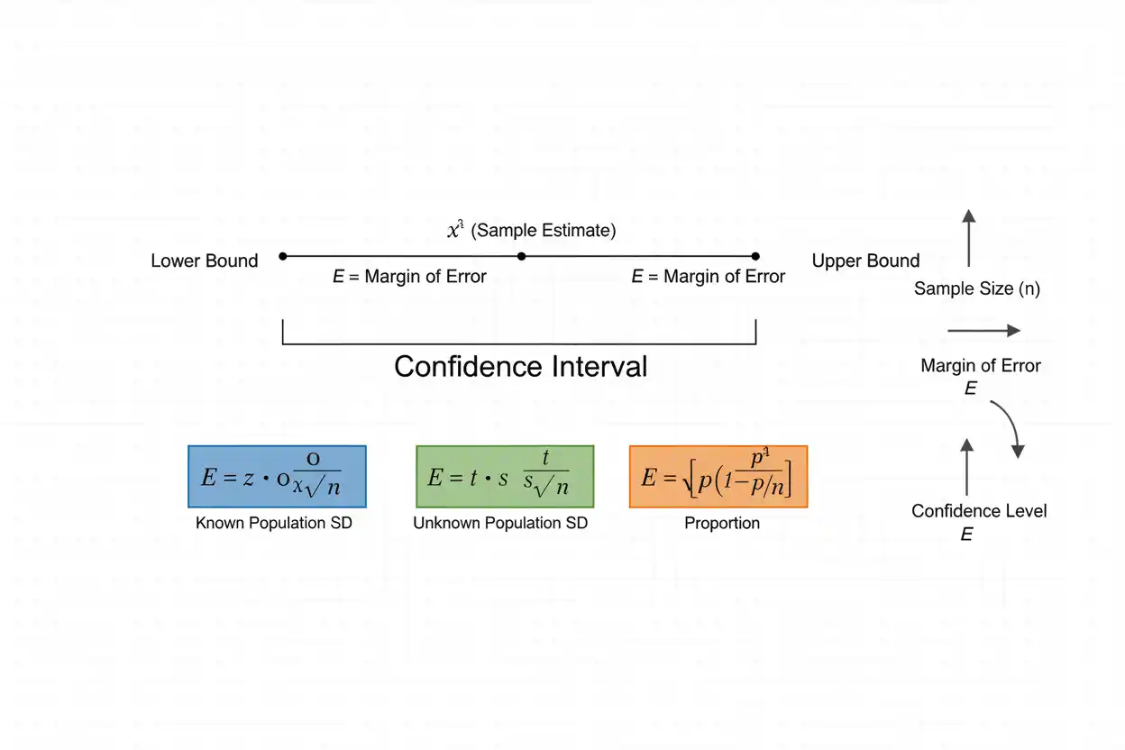
The margin of error is a statistical quantity that measures how far an interval estimate extends from a sample-based point estimate under a specified confidence procedure, providing a practical expression of sampling uncertainty in the same units as the estimated parameter. In the familiar form estimate ± margin of error, the margin of error is commonly calculated as a critical value multiplied by the standard error, so it becomes larger when greater confidence is required or sampling variability is high and becomes smaller when the estimate is based on more information. For a population mean with known standard deviation, for example, a common normal-theory formula is E = zσ/√n, while a mean with unknown population standard deviation commonly uses E = ts/√n under the appropriate t-based assumptions. Proportion estimates use a different standard-error formula, and more complex sampling designs can require weighting, clustering adjustments, or finite-population corrections. Most importantly, margin of error measures uncertainty represented by the sampling model; it does not automatically account for biased sampling, measurement error, nonresponse, incorrect models, or other systematic errors that can move an estimate away from the population value.
Within descriptive statistics and the broader Statistics & Probability framework, margin of error connects observed sample information with inferential precision. Understanding that connection helps explain why a study can have a very small margin of error yet still be inaccurate if its data collection is biased, and why a wider margin is sometimes the statistically appropriate reflection of limited information rather than a defect in the analysis.
What Is Margin of Error?
Margin of error is the distance between a point estimate and either endpoint of a symmetric confidence interval.
If an estimate is:
50
with margin of error:
4
the interval is:
50 ± 4
which gives:
Lower bound = 46
Upper bound = 54
The margin of error is therefore:
E = 4.
It represents uncertainty around the estimated parameter under the specified confidence procedure.
It does not mean every observed value lies within four units of 50.
General Margin of Error Formula
A broad form is:
E = Critical value × Standard error
Therefore:
Interval = Estimate ± E
and:
Lower bound = Estimate − E
Upper bound = Estimate + E
The exact critical value and standard-error formula depend on:
- the parameter being estimated;
- the sampling distribution;
- sample size;
- known or estimated population variability;
- confidence level;
- sampling design.
Thus, there is no single margin-of-error formula appropriate for every statistical problem.
Components of Margin of Error
Three ideas determine most elementary margin-of-error calculations.
The first is the standard error, which quantifies how much the estimator varies from sample to sample.
The second is the critical value, which specifies how many standard errors the interval extends from the estimate.
The third is the confidence level, which determines the long-run coverage target and therefore influences the critical value.
For example:
E = 1.96 × 2
gives:
E = 3.92.
Here:
2
is the standard error, while:
1.96
is the critical value for a common 95% standard-normal procedure.
Margin of Error for a Mean With Known Population Standard Deviation
When estimating a population mean μ and the population standard deviation σ is known, a common margin-of-error formula is:
E = z*σ/√n
where:
- E = margin of error
- z* = standard-normal critical value
- σ = population standard deviation
- n = sample size
The corresponding interval is:
x̄ ± z*σ/√n
under the assumptions supporting the normal procedure.
Because n appears under a square root, increasing sample size reduces uncertainty, but not in direct one-for-one proportion.
Known-σ Example
Suppose:
σ = 15
n = 100
and a 95% confidence procedure is used.
The standard error is:
SE = 15/√100
= 15/10
= 1.5
For 95% confidence:
z* ≈ 1.96
Therefore:
E = 1.96(1.5)
= 2.94
The margin of error is:
2.94 units.
If the sample mean were:
x̄ = 80
the corresponding interval would be:
80 ± 2.94
or:
(77.06, 82.94)
Margin of Error When σ Is Unknown
Population standard deviation is rarely known exactly.
When estimating a mean from a sample and σ is unknown, a common classical procedure uses:
E = t*s/√n
where:
- s = sample standard deviation
- t* = critical value from Student’s t distribution
- degrees of freedom = n − 1
The corresponding interval is:
x̄ ± t*s/√n.
The t critical value is generally larger than the equivalent standard-normal critical value for finite samples because σ itself has been estimated.
t-Based Margin of Error Example
Suppose:
n = 25
s = 10
and a 95% confidence interval for the population mean is required.
Degrees of freedom are:
df = 25 − 1
= 24
The 95% two-sided t critical value is approximately:
t* = 2.064
The standard error is:
SE = 10/√25
= 10/5
= 2
Therefore:
E = 2.064(2)
= 4.128
So the margin of error is approximately:
4.13 units.
Why t Gives a Larger Margin Than z
If the same standard error:
SE = 2
were multiplied by:
z* = 1.96
the margin would be:
E = 3.92.
Using:
t* = 2.064
instead produces:
E = 4.128.
The additional width reflects uncertainty caused by estimating the unknown population standard deviation from the sample.
As sample size increases, the t critical value approaches its standard-normal counterpart.
Therefore, the numerical difference becomes increasingly small.
Margin of Error for a Population Proportion
For a sample proportion:
p̂ = x/n
a commonly taught large-sample normal approximation uses:
E = z*√[p̂(1−p̂)/n]
The associated interval is:
p̂ ± E.
This formula is intuitive and useful for understanding sampling precision, although the resulting Wald interval can perform poorly for small samples or proportions near:
0
or:
Methods such as the Wilson interval are often preferable in those settings.
Proportion Margin of Error Example
Suppose:
n = 400
and:
p̂ = 0.60.
For a 95% normal approximation:
z* = 1.96
Calculate the estimated standard error:
SE = √[(0.60)(0.40)/400]
= √(0.24/400)
= √0.0006
≈ 0.024495
Therefore:
E = 1.96(0.024495)
≈ 0.0480
The margin of error is approximately:
0.048
or:
4.8 percentage points.
The approximate interval is therefore:
60% ± 4.8 percentage points
or:
55.2% to 64.8%.
Percentage Points vs Percent
Margin of error for a percentage estimate is usually best expressed in percentage points.
If:
Estimate = 60%
and:
E = 4.8 percentage points
then the interval is:
55.2% to 64.8%.
It would be misleading to describe the margin simply as:
4.8%
if readers might interpret that as 4.8% of 60.
A relative 4.8% change from 60% would equal only:
0.048 × 60% = 2.88 percentage points.
Percentage points avoid that ambiguity.
Common z Critical Values
For two-sided standard-normal confidence procedures, commonly used values include:
| Confidence Level | z* |
|---|---|
| 80% | 1.282 |
| 90% | 1.645 |
| 95% | 1.960 |
| 98% | 2.326 |
| 99% | 2.576 |
Higher confidence requires a larger critical value.
Therefore, with sample size and standard error unchanged:
Higher confidence → larger margin of error
while:
Lower confidence → smaller margin of error.
This is one of the fundamental precision-confidence tradeoffs in interval estimation.
Effect of Confidence Level
Suppose:
SE = 5.
At 90% confidence:
E = 1.645(5)
= 8.225
At 95% confidence:
E = 1.96(5)
= 9.8
At 99% confidence:
E = 2.576(5)
= 12.88
Thus:
90% margin = 8.225
95% margin = 9.8
99% margin = 12.88
The same sample produces wider uncertainty bounds when the procedure is designed for higher long-run coverage.
Confidence vs Precision
Higher confidence and narrower margins are both desirable in isolation, but for fixed data they conflict.
To increase confidence while keeping everything else fixed, the critical value must increase.
That widens the margin.
To preserve the same margin at a higher confidence level, more information—usually a larger sample—is required.
This is why statements such as “we want 99.9% confidence and almost no margin of error” can imply a very large data requirement.
Precision has a cost.
Effect of Sample Size
For a mean with fixed σ:
E = z*σ/√n.
Therefore:
E ∝ 1/√n.
If sample size increases from:
n = 100
to:
n = 400,
then:
√100 = 10
and:
√400 = 20.
The denominator doubles, so the margin of error is cut in half.
This square-root relationship is one of the most important rules in sample-size planning.
Doubling Sample Size
Doubling sample size does not halve the margin of error.
If:
n → 2n,
then:
E_new/E_old = 1/√2
≈ 0.707.
Therefore, the margin decreases by approximately:
29.3%.
For example, a margin of:
10
would fall to approximately:
7.07
after doubling n, assuming variability and confidence level remain unchanged.
To halve the margin, sample size generally must be multiplied by four.
Quadrupling Sample Size
Suppose:
n = 100
produces:
E = 6.
If everything except sample size remains constant and:
n = 400,
then:
E_new = 6 × √(100/400)
= 6 × 1/2
= 3.
Thus:
4× sample size → 1/2 margin of error.
This relationship explains why extremely small desired margins can require dramatically larger studies.
Effect of Variability
For a population mean:
E = Critical value × Standard deviation/√n.
Therefore, greater variability produces greater uncertainty.
Suppose two populations are sampled using the same:
n = 100
and:
z* = 1.96.
If Population A has:
σ = 10
then:
E_A = 1.96.
If Population B has:
σ = 30
then:
E_B = 5.88.
The second population requires a larger sample to estimate its mean with the same margin.
Why Variable Data Need More Information
If observations are tightly concentrated, a sample mean tends to vary less between samples.
If observations are widely dispersed, different samples can produce substantially different means.
Standard error captures this distinction.
Therefore:
greater observation-level variability
usually creates:
greater estimator uncertainty.
This is why understanding distribution shape through tools such as a histogram can be useful before interpreting inferential precision, especially when unusually dispersed or extreme observations influence the standard deviation.
Margin of Error and Kurtosis
Kurtosis is not part of the elementary margin-of-error formula directly, but heavy-tail behavior can matter indirectly because extreme observations can inflate variability and make simple normal approximations less stable in modest samples.
For example, a distribution containing rare but extreme observations can produce a highly variable sample mean and sample standard deviation.
A formula such as:
t*s/√n
will reflect the observed increase in s, but a small sample may still provide limited information about the true tail structure.
Therefore, distributional assumptions should accompany—not be replaced by—the numerical margin.
Margin of Error and the Median
The median is a positional measure of center, while many familiar margin-of-error formulas are derived specifically for means or proportions.
A formula such as:
z*σ/√n
should not be attached automatically to the median.
Confidence intervals for population medians can instead use:
- order-statistic methods;
- quantile methods;
- bootstrap procedures;
- distribution-specific approximations.
The term margin of error can still be used informally for half the width of a symmetric median interval, but the calculation must match the estimator’s sampling distribution.
Margin of Error and Median Absolute Deviation
The median absolute deviation is a robust measure of spread centered on the median, whereas ordinary mean-based margin-of-error formulas typically use standard deviation or a standard error derived from variance.
The two concepts serve different purposes.
MAD describes the dispersion of observed data robustly.
Margin of error describes uncertainty in an estimated parameter.
Robust inferential procedures can use MAD-related scale estimators in specialized settings, but one should not substitute MAD mechanically for σ or s in a textbook standard-error formula without deriving or specifying the corresponding method.
Margin of Error and Harmonic Mean
The harmonic mean is useful for certain rate and reciprocal-average problems, but its uncertainty does not generally follow the ordinary sample-mean standard-error formula without additional analysis.
Because the harmonic mean depends on reciprocals:
H = n/Σ(1/xᵢ),
values near zero can create substantial sampling instability.
If a population harmonic mean is being estimated, a valid margin of error should come from the sampling behavior of that estimator, potentially through analytical approximations, transformations, or resampling.
The standard arithmetic-mean formula should not be reused automatically.
Margin of Error Is Not Standard Deviation
Standard deviation measures variation among individual observations.
Margin of error measures uncertainty in an estimated parameter.
Suppose:
σ = 20
and:
n = 100.
The standard error of the mean is:
20/√100
= 2.
A 95% z margin is:
1.96(2)
= 3.92.
Therefore:
SD = 20
while:
Margin of error = 3.92.
They are related but clearly not the same quantity.
Margin of Error Is Not Standard Error
Standard error is one component of margin of error.
The relationship is:
E = Critical value × SE.
Suppose:
SE = 2.5
and:
z* = 1.96.
Then:
E = 4.9.
Thus:
Standard error = 2.5
while:
Margin of error = 4.9.
The standard error describes one standard-deviation unit of sampling uncertainty, whereas the margin extends far enough to achieve the selected confidence coverage under the interval procedure.
Margin of Error Is Not the Confidence Level
A confidence level might be:
95%.
A margin of error might be:
±3 percentage points.
These numbers represent different concepts.
Confidence level describes the long-run coverage target.
Margin of error describes interval half-width.
A survey statement such as:
“60% ±3 percentage points at 95% confidence”
contains both quantities and should not conflate them.
Margin of Error and Interval Width
For a symmetric interval:
Lower = Estimate − E
Upper = Estimate + E.
Therefore:
Interval width = Upper − Lower
= 2E.
So:
E = Interval width/2.
If an interval is:
(40, 50),
its width is:
10
and its margin of error is:
This shortcut works only for intervals symmetric around the point estimate.
Asymmetric Confidence Intervals
Not every inferential interval is symmetric.
Suppose an interval is:
(2, 10)
around a point estimate of:
The distances are:
5 − 2 = 3
and:
10 − 5 = 5.
There is no single common half-width.
In such cases, reporting:
lower error = 3
upper error = 5
can be clearer than forcing the result into a symmetric ±E form.
This occurs frequently with transformed parameters, ratios, variances, and some bootstrap procedures.
Margin of Error From an Existing Symmetric Interval
Suppose a report gives:
Estimate = 72
95% interval = (68, 76).
Then:
E = 76 − 72
= 4
and:
E = 72 − 68
= 4.
Alternatively:
E = (76 − 68)/2
= 4.
Therefore:
Margin of error = 4.
This is useful when the interval is reported but the margin is not.
Margin of Error From Lower and Upper Bounds
For a symmetric interval:
E = (Upper − Lower)/2.
The midpoint is:
Estimate = (Upper + Lower)/2.
Suppose:
Lower = 91.2
Upper = 96.8.
Then:
Estimate = (91.2 + 96.8)/2
= 94
and:
E = (96.8 − 91.2)/2
= 2.8.
The result can therefore be written:
94 ± 2.8.
Margin of Error for Polling
Poll results are often reported in a form such as:
52% ±3 percentage points.
This usually represents a sampling-based interval around an estimated proportion under a stated or implied confidence level.
However, the published margin may incorporate:
- weighting;
- survey design effects;
- effective sample size;
- rounding.
It also does not automatically account for:
- nonresponse bias;
- question wording;
- coverage error;
- turnout modeling;
- measurement error.
Therefore, “±3” is not a guarantee that the true value is within three points.
Maximum Proportion Margin of Error
For the simple proportion formula:
E = z*√[p(1−p)/n],
the expression:
p(1−p)
is maximized at:
p = 0.5.
At p = 0.5:
p(1−p) = 0.25.
Therefore, when no prior estimate is available, a conservative planning formula is:
E = z*√(0.25/n)
or:
E = z*/(2√n).
This produces the largest standard error under the simple binomial model for a fixed n.
Example of Maximum Proportion Margin
Suppose:
n = 1,000
and:
z* = 1.96.
Using:
p = 0.5
gives:
E = 1.96√(0.25/1000)
= 1.96√0.00025
= 1.96(0.015811)
≈ 0.03099.
Thus, the approximate maximum 95% sampling margin is:
3.10 percentage points.
A sample proportion farther from 0.5 would produce a slightly smaller simple Wald standard error.
Why 50% Produces the Largest Proportion Variance
For a Bernoulli variable:
Var(X) = p(1−p).
This quadratic is largest when:
p = 0.5.
For example:
p = 0.5 → p(1−p) = 0.25
while:
p = 0.9 → p(1−p) = 0.09.
Thus, binary outcomes are most variable when successes and failures are equally likely.
This makes 50% a conservative planning choice when the true population proportion is unknown.
Sample Size for a Desired Mean Margin of Error
For a mean with known or planned σ:
E = z*σ/√n.
Solve for n:
√n = z*σ/E
and:
n = (z*σ/E)².
Suppose:
σ = 12
E = 3
z* = 1.96.
Then:
n = [1.96(12)/3]²
= (7.84)²
= 61.4656.
Round upward:
n = 62.
A sample size of at least 62 is required under this planning formula.
Why Sample Size Is Rounded Up
Suppose the formula yields:
n = 61.47.
Using:
n = 61
would produce a slightly larger margin than requested.
Using:
n = 62
meets or exceeds the precision target under the assumptions.
Therefore, sample-size calculations are normally rounded upward rather than to the nearest whole number.
Precision requirements create minimum sample sizes.
Sample Size for a Proportion
A simple planning formula is:
n = z*²p(1−p)/E².
If p is unknown, use:
p = 0.5.
Suppose the target is:
95% confidence
with margin:
E = 0.05.
Then:
n = 1.96²(0.25)/(0.05²)
= 3.8416(0.25)/0.0025
= 0.9604/0.0025
= 384.16.
Round upward:
n = 385.
This is the familiar simple-random-sampling planning result before design or finite-population adjustments.
Reducing Margin of Error From 5% to 2.5%
Because:
n ∝ 1/E²,
halving E requires four times as many observations.
If approximately:
n = 385
gives a five-percentage-point maximum margin, then roughly:
4 × 385
= 1,540
observations are required for about:
2.5 percentage points,
under otherwise identical assumptions.
Very tight margins therefore increase sample requirements rapidly.
Finite Population Correction
When sampling without replacement from a finite population and the sample constitutes a substantial fraction of that population, the standard error can be reduced with the finite population correction:
FPC = √[(N − n)/(N − 1)]
where:
- N = population size
- n = sample size
For a mean, a corrected standard error can be written:
SE = σ/√n × FPC
under simple random sampling without replacement.
The corresponding margin is:
E = Critical value × SE.
Finite Population Example
Suppose:
N = 1,000
n = 400.
Then:
FPC = √[(1000 − 400)/(1000 − 1)]
= √(600/999)
≈ 0.775.
Without the correction, suppose:
SE = 2.
The corrected standard error is approximately:
2(0.775)
= 1.55.
A 95% normal margin becomes:
E ≈ 1.96(1.55)
≈ 3.04
instead of:
3.92.
Sampling 40% of a finite population provides more information than treating the population as effectively infinite.
When Finite Population Correction Is Small
If:
n/N
is tiny, then:
N − n ≈ N
and:
FPC ≈ 1.
For example, sampling:
1,000
people from a population of:
100,000,000
makes the correction effectively negligible.
This is why many large-population survey formulas depend primarily on sample size rather than the total population size.
Once the population is very large relative to n, adding millions more population members changes sampling precision very little.
Population Size Does Not Directly Determine Margin in Large Populations
A common misconception is that a country with 100 million people necessarily requires a dramatically larger survey than a city with one million people to achieve the same simple-random-sampling margin of error.
When both populations are very large relative to the sample, the finite-population correction is nearly one.
The key drivers are instead:
- sample size;
- confidence level;
- population variability;
- sampling design.
Population size becomes important primarily when sampling a substantial fraction of the population.
Design Effect
Complex sampling can change precision compared with simple random sampling.
A design effect is often expressed as:
DEFF = Var_complex / Var_SRS.
If:
DEFF = 2,
the variance is twice the simple-random-sample variance.
Because standard error is the square root of variance:
SE_complex = √2 × SE_SRS
≈ 1.414 × SE_SRS.
The margin of error likewise increases by approximately:
41.4%
if the same critical value applies.
Effective Sample Size
Design effect can be translated approximately into effective sample size:
n_eff ≈ n/DEFF.
Suppose:
n = 2,000
but:
DEFF = 2.
Then:
n_eff ≈ 1,000.
In terms of variance, the complex sample provides approximately the precision of a simple random sample containing 1,000 independent observations.
This is why quoting only the raw number of survey respondents can exaggerate apparent precision when clustering or weighting is substantial.
Cluster Sampling
When observations inside a cluster resemble one another, each additional observation can provide less new information than an independent observation would.
For example, surveying many people within a small number of households, schools, or geographic areas can create positive intracluster correlation.
Ignoring that structure can underestimate the standard error and therefore produce an unrealistically small margin.
Cluster-aware variance estimation is required.
The nominal sample size by itself does not determine inferential precision.
Stratified Sampling
Stratification can sometimes improve precision when the population is divided into internally homogeneous strata and sampling is designed appropriately.
The overall variance then depends on:
- stratum sizes;
- within-stratum variability;
- sample allocation.
A correctly designed stratified sample can produce a smaller margin than a simple random sample of the same total size.
However, the exact formula differs from the elementary one-sample expression.
The variance calculation must match the design.
Weighting
Survey or observational analyses often use weights because observations represent unequal population amounts or because adjustments are made for sampling probabilities and nonresponse.
Unequal weights can increase variance.
A weighted estimate may therefore have a larger standard error than an unweighted estimate based on the same nominal n.
The corresponding margin of error should be calculated from a variance estimator appropriate to the weights.
Simply applying:
1.96√[p̂(1−p̂)/n]
to a heavily weighted sample can understate uncertainty.
One-Sided Margin of Error
Sometimes the objective is an upper or lower confidence bound rather than a two-sided interval.
For a one-sided 95% standard-normal bound, the critical value is approximately:
1.645
rather than:
1.96.
For example:
Upper bound = Estimate + 1.645(SE)
provides a common one-sided 95% procedure under normal assumptions.
The required critical value depends on how α is allocated.
Therefore, “95% confidence” alone does not specify the multiplier unless one knows whether the procedure is one-sided or two-sided.
Alpha and Margin of Error
For a two-sided confidence interval:
Confidence level = 1 − α.
At:
95% confidence
we have:
α = 0.05.
The two tails typically contain:
α/2 = 0.025
each.
The critical value therefore satisfies:
P(−z* ≤ Z ≤ z*) = 0.95.
For the standard normal:
z* ≈ 1.96.
Understanding α helps explain why higher confidence requires larger critical values.
Margin of Error and Statistical Significance
For a symmetric confidence interval around an estimated difference:
Estimate ± E,
the value zero is excluded when:
|Estimate| > E.
For example:
Estimated difference = 5
Margin = 2
gives:
(3, 7),
which excludes zero.
A matching two-sided test would reject a zero-difference null at the corresponding significance level when assumptions and methods align.
However, statistical significance does not establish that the difference is practically important.
Statistical Significance vs Practical Importance
Suppose a very large sample estimates a difference of:
0.10 units
with margin of error:
0.02.
The interval:
(0.08, 0.12)
excludes zero clearly.
The effect may therefore be statistically detectable.
Yet a difference of:
0.10 units
could be operationally trivial.
A small margin of error indicates precision, not importance.
The magnitude must be interpreted in the context of the problem.
Margin of Error Does Not Measure Bias
Suppose a thermometer consistently reads:
5°C too high.
A large number of repeated measurements may produce a tiny sampling margin around the average reading.
The result can be:
highly precise
but:
systematically wrong.
Margin of error quantifies uncertainty from the variation represented in the statistical procedure.
It does not automatically correct a systematic measurement bias.
Precision and accuracy are separate concepts.
Sampling Bias
Suppose an election survey excludes an important segment of the population.
Even if:
n = 100,000,
the sampling margin could be numerically tiny.
However, if the excluded group differs systematically from the included respondents, the estimate can remain biased.
Increasing n reduces random error around the biased sampling mechanism.
It does not make the sample representative.
Therefore, a tiny reported margin should never be interpreted as proof of an unbiased estimate.
Nonresponse Bias
A survey can randomly select an excellent probability sample but still suffer bias if many selected people do not respond and response propensity is related to the measured outcome.
The ordinary sampling margin typically does not capture this systematic nonresponse mechanism automatically.
Weighting and modeling may reduce the problem, but those methods bring their own assumptions.
Thus:
Sampling error ≠ total survey error.
The reported ± figure is only one part of overall uncertainty.
Measurement Error
Suppose respondents misunderstand a question or an instrument records values imprecisely.
These errors can affect estimates even when sampling uncertainty is small.
If measurement noise behaves randomly, it may increase observed variability.
If measurement error is systematic, it can shift the estimate itself.
The ordinary margin of error may not fully represent either mechanism unless the statistical model explicitly incorporates it.
High-quality measurement therefore matters just as much as sample size.
Model Error
Many margins rely on assumptions such as:
- independence;
- correct sampling design;
- valid variance formula;
- approximate distributional behavior.
If those assumptions are badly wrong, the nominal confidence level may not reflect actual coverage.
A margin of:
±2
is only meaningful relative to the method that generated it.
Statistical uncertainty cannot be separated from model validity.
Missing Data
Missing observations can reduce effective sample size and potentially introduce bias.
If values are missing completely at random, the main effect may be a larger standard error because fewer observations remain.
If missingness is systematically related to the outcome, the point estimate itself can become biased.
A conventional margin calculated only from observed data may then describe random uncertainty around a distorted estimate.
The missing-data process should therefore be considered explicitly.
Outliers and Margin of Error
Extreme observations can increase:
s
and therefore increase:
s/√n.
Consequently:
E = t*s/√n
can become wider.
This is not necessarily a problem with the formula.
If the extreme observation genuinely belongs to the population, the greater variability represents real uncertainty.
Removing it merely to shrink the margin would understate the variability of the process.
Outliers should be investigated, not mechanically discarded.
Robust Alternatives
When a population is highly skewed or contaminated by extreme observations, robust estimators may provide a more appropriate target than the ordinary mean.
Examples can include:
- trimmed means;
- medians;
- robust location estimators.
Their confidence intervals can be constructed using:
- asymptotic theory;
- order statistics;
- bootstrap methods.
The resulting “margin of error” may not have the simple:
t*s/√n
form.
The formula should follow the estimator rather than the other way around.
Bootstrap Margin of Error
Bootstrap resampling can estimate the sampling distribution of a statistic.
A simple workflow is:
- repeatedly resample observations with replacement;
- calculate the statistic for each resample;
- measure the variability of the bootstrap estimates;
- construct an interval using an appropriate bootstrap method.
If a symmetric bootstrap interval is:
Estimate ± E,
its half-width can be described as a bootstrap margin of error.
However, many bootstrap intervals are asymmetric, in which case separate lower and upper uncertainties are clearer.
Margin of Error for Regression Coefficients
Suppose an estimated regression coefficient is:
b = 2.4
with:
SE(b) = 0.5.
If the appropriate two-sided critical value is:
t* = 2.05,
then:
E = 2.05(0.5)
= 1.025.
The interval is:
2.4 ± 1.025
or:
(1.375, 3.425).
The same general structure applies:
Estimate ± Critical value × Standard error,
although the standard error arises from the regression model rather than a simple raw sample mean.
Margin of Error for a Difference Between Means
For two independent groups, an estimated difference is:
x̄₁ − x̄₂.
A Welch-type standard error is:
SE = √(s₁²/n₁ + s₂²/n₂).
The margin is:
E = t*SE
using appropriate degrees of freedom.
Suppose:
SE = 2.3
and:
t* = 2.0.
Then:
E ≈ 4.6.
If the estimated difference is:
7,
the interval is approximately:
7 ± 4.6
or:
(2.4, 11.6).
Paired Data
For paired observations, uncertainty should be calculated from the paired differences.
If:
dᵢ = beforeᵢ − afterᵢ,
then:
d̄
is the estimated mean difference and:
SE(d̄) = s_d/√n.
The margin is:
E = t*s_d/√n.
Treating the two paired samples as independent can inflate or understate uncertainty depending on the within-pair relationship.
The standard-error formula must respect the study design.
Margin of Error and Repeated Measurements
Repeated observations from the same individual are generally correlated.
Treating 100 repeated measurements from one person as though they were 100 independent people can make:
n
appear much larger than the effective information content.
This can produce an artificially small margin.
Repeated-measures, mixed-model, or cluster-aware methods are designed to represent such dependence.
Independence is an assumption with practical consequences, not merely a mathematical convenience.
Margin of Error for Finite Population Proportions
A simple proportion standard error under sampling without replacement can be multiplied by the finite population correction:
SE = √[p̂(1−p̂)/n] × √[(N−n)/(N−1)]
under the corresponding simple design.
Then:
E = z*SE.
If the sampling fraction:
n/N
is substantial, the correction can materially reduce the margin.
If the fraction is tiny, the effect is negligible.
Can Margin of Error Be Zero?
A calculated sampling margin can be zero in special circumstances, such as a finite population being completely observed with no remaining sampling uncertainty under the target estimand.
In ordinary sample-based settings, exactly zero margin would generally require:
zero standard error
or:
zero critical value.
A zero standard error can occur in degenerate data under some simple calculations, but it does not necessarily mean every relevant source of uncertainty is absent.
Systematic measurement and modeling uncertainty can remain.
Can Margin of Error Be Larger Than the Estimate?
Yes.
Suppose:
Estimate = 2
and:
E = 5.
The symmetric interval is:
(−3, 7).
This may be entirely legitimate if the parameter can take negative values.
For a parameter constrained to nonnegative values, however, an interval method respecting that parameter space may be preferable.
A large margin relative to the estimate indicates low precision, not necessarily a calculation error.
Margin of Error Near Parameter Boundaries
For proportions:
0 ≤ p ≤ 1.
A simple symmetric interval can produce impossible endpoints.
For example:
p̂ = 0.03
with:
E = 0.05
would give:
(−0.02, 0.08).
The negative endpoint cannot represent a true probability.
This demonstrates why methods such as Wilson or exact binomial intervals are useful near boundaries.
The concept of sampling uncertainty remains valid, but the interval construction should respect the parameter’s mathematical limits.
Rounding Margin of Error
Intermediate calculations should retain adequate precision.
Suppose:
SE = 1.76438
and:
z* = 1.96.
Calculate:
E = 3.45818
before rounding.
A sensible report might be:
E ≈ 3.46.
Rounding the standard error too early can shift the final endpoints.
The margin and estimate should also use compatible decimal precision.
Reporting Estimate ± Margin
Suppose:
Estimate = 47.6
E = 2.3.
A concise report is:
47.6 ± 2.3
with the confidence level and method stated nearby.
The implied interval is:
(45.3, 49.9).
Without the confidence level, however, the ± value is incomplete because the same standard error would produce different margins at 90%, 95%, and 99% confidence.
Always connect the margin to its inferential context.
Full Worked Mean Example
Suppose a random sample gives:
x̄ = 72
σ = 16
n = 64
and a 95% confidence procedure is used.
Step 1: Calculate Standard Error
SE = σ/√n
= 16/√64
= 16/8
= 2
Step 2: Find the Critical Value
z* = 1.96
Step 3: Calculate Margin of Error
E = 1.96(2)
= 3.92
Step 4: Construct the Interval
72 ± 3.92
Therefore:
Lower = 68.08
Upper = 75.92
The 95% margin of error is:
3.92 units.
Full Worked t Example
Suppose:
x̄ = 40
s = 6
n = 16.
For a classical 95% t interval:
df = 15
and:
t* ≈ 2.131.
Standard error:
SE = 6/√16
= 1.5.
Margin:
E = 2.131(1.5)
= 3.1965.
Therefore:
E ≈ 3.20.
The confidence interval is:
40 ± 3.20
or approximately:
(36.80, 43.20).
Full Worked Proportion Example
Suppose a sample of:
n = 600
contains:
x = 330
successes.
Then:
p̂ = 330/600
= 0.55.
Estimated standard error:
SE = √[(0.55)(0.45)/600]
= √(0.2475/600)
= √0.0004125
≈ 0.02031.
At 95% confidence:
E = 1.96(0.02031)
≈ 0.0398.
Thus, the approximate margin is:
3.98 percentage points.
The corresponding simple interval is approximately:
51.02% to 58.98%.
Comparing Two Studies
Suppose Study A reports:
Estimate = 50
E = 10.
Study B reports:
Estimate = 50
E = 2.
The point estimates are identical.
Study B is much more precise under its stated procedure because its interval is narrower.
However, this does not prove Study B has a better sampling design.
Its small margin could result from a huge but biased sample.
Precision must be considered alongside validity.
Why a Very Small Margin Can Mislead
Suppose an online poll receives:
1,000,000
voluntary responses.
A naïve random-sampling formula could imply an extremely small standard error.
But voluntary participation can create strong selection bias.
A much smaller genuinely randomized sample could estimate the target population more accurately despite having a larger sampling margin.
Margin of error measures one dimension of uncertainty.
It is not a substitute for sound data collection.
Margin of Error and Data Distribution
Two samples can have the same mean but different margins because their variability differs.
A sample concentrated tightly around its mean produces smaller:
s
and therefore smaller:
SE = s/√n.
A dispersed sample produces larger uncertainty.
Graphical inspection is useful because one large s can arise from:
- broad ordinary variation;
- skewness;
- one extreme observation;
- several subgroups.
The numerical standard error alone does not reveal which mechanism is responsible.
Margin of Error and Robust Spread
When extreme values dominate standard deviation, robust descriptive quantities can provide useful context even if the inferential target remains the population mean.
For example, comparing:
standard deviation
with:
median absolute deviation
can reveal whether ordinary variance is being driven strongly by tails.
This does not mean the robust spread should be substituted directly into a classical t formula.
It means distributional diagnostics can help determine whether the assumed procedure is appropriate.
Common Margin of Error Mistakes
A common mistake is treating margin of error as the maximum possible difference between an estimate and the truth. Confidence procedures allow noncoverage, and systematic errors can place the true parameter farther away than the reported sampling margin.
Another mistake is assuming that ±5% means ±5% relative to the estimate when survey reports often mean ±5 percentage points.
Analysts also sometimes use:
1.96
automatically for every 95% interval, even when the problem requires a t critical value, another probability distribution, or an asymmetric method.
Another error is believing that doubling sample size halves the margin; the relationship usually follows:
1/√n.
Ignoring clustering, weighting, finite-population structure, or paired observations can also produce incorrect standard errors.
A particularly serious mistake is interpreting a tiny margin as proof of accuracy when sampling bias, measurement error, or model error may remain.
Finally, margin of error should not be confused with standard deviation, standard error, confidence level, prediction error, or the spread of individual observations.
How to Calculate Margin of Error Step by Step
Begin by identifying the parameter being estimated and the statistical procedure appropriate for it.
Next calculate or estimate the standard error.
For a known-σ mean:
SE = σ/√n.
For a t-based sample mean:
SE = s/√n.
For a simple sample proportion:
SE ≈ √[p̂(1−p̂)/n].
Choose the confidence level and appropriate critical value.
Then calculate:
E = Critical value × SE.
Finally, construct the interval if it is symmetric:
Estimate ± E
and interpret the margin strictly in the context of the sampling method and assumptions used.
When Margin of Error Is Most Useful
Margin of error is particularly useful when a reader needs a concise measure of precision around an estimate.
It can help compare:
- survey proportions;
- estimated means;
- group differences;
- model coefficients;
- other approximately symmetric interval estimates.
It also makes sample-size tradeoffs easy to communicate.
However, it is most informative when reported alongside:
- confidence level;
- sample size;
- point estimate;
- sampling method.
A bare ± number lacks essential context.
When Margin of Error Needs Additional Caution
Interpretation deserves extra care when:
- the sample is nonrandom;
- response rates are low;
- observations are dependent;
- weights vary substantially;
- sample size is very small;
- the population is highly skewed or heavy-tailed;
- the parameter lies near a natural boundary;
- the interval method is asymmetric;
- measurement error dominates sampling error.
In such situations, a textbook formula can give a numerically precise answer without representing all important uncertainty.
The procedure should match the structure of the data.
How to Report Margin of Error
A clear report might state:
“The estimated mean was 72 units, with a 95% margin of error of 3.92 units, corresponding to an interval from 68.08 to 75.92.”
For a proportion:
“The estimated proportion was 55%, with an approximate 95% margin of error of 3.98 percentage points.”
For complex surveys, reporting the method or design-adjusted standard error can be important.
Avoid implying that the margin covers every possible source of error.
It is best described as a measure of statistical precision under the specified procedure.
Frequently Asked Questions About Margin of Error
What is margin of error?
Margin of error is the distance from a point estimate to the boundary of a symmetric confidence interval under a specified statistical procedure.
What is the general formula?
E = Critical value × Standard error
What is the mean formula when σ is known?
E = z*σ/√n
What is the mean formula when σ is unknown?
A common classical formula is:
E = t*s/√n
What is the formula for a sample proportion?
A common large-sample approximation is:
E = z*√[p̂(1−p̂)/n]
What does ±3 mean?
It means the symmetric interval extends three units below and three units above the point estimate.
Is margin of error the same as confidence level?
No. Confidence level is a coverage percentage; margin of error is an interval half-width.
Is margin of error the same as standard error?
No. Margin of error equals a critical value multiplied by standard error.
Is margin of error the same as standard deviation?
No. Standard deviation describes individual-data variability, while margin of error describes estimator precision.
What is the 95% z critical value?
Approximately:
1.96.
What is the 90% z critical value?
Approximately:
1.645.
What is the 99% z critical value?
Approximately:
2.576.
Does higher confidence increase margin of error?
Yes, when the sample and method remain unchanged.
Does a larger sample reduce margin of error?
Generally yes.
How does margin of error change with n?
For many elementary estimators:
E ∝ 1/√n.
Does doubling sample size halve margin of error?
No. It multiplies it by approximately:
1/√2 ≈ 0.707.
How do you halve margin of error?
Approximately quadruple the sample size, all else equal.
Does larger standard deviation increase margin of error?
Yes.
Why?
Greater data variability increases the standard error of the mean.
Can margin of error be expressed in percentage points?
Yes, and this is common for estimated proportions.
Is ±5 percentage points the same as ±5% relative error?
No.
Why is p = 0.5 used in proportion sample-size planning?
Because:
p(1−p)
is maximized at 0.25 when p = 0.5.
What is the conservative proportion sample-size formula?
n = z*²(0.25)/E²
when p is unknown.
Do large populations always require larger samples?
No. Once population size is very large relative to n, the sampling margin depends much more on n than on total population size.
What is finite population correction?
√[(N−n)/(N−1)]
for common simple-random-sampling settings.
When does finite population correction matter?
When the sample is a substantial fraction of the finite population.
What is design effect?
It compares the sampling variance under a complex design with that under simple random sampling.
How does design effect change the margin?
If:
DEFF > 1,
the standard error and margin generally increase by approximately:
√DEFF.
What is effective sample size?
A rough relationship is:
n_eff ≈ n/DEFF.
Does a small margin prove a survey is accurate?
No.
Why not?
Sampling bias, nonresponse, measurement error, and model error can remain even when sampling precision is extremely high.
Can a biased estimate have a tiny margin of error?
Yes.
Does margin of error include all survey errors?
No. It usually represents sampling uncertainty under a particular model or design.
Do outliers affect margin of error?
They can, especially for mean-based procedures because outliers can increase sample standard deviation.
Should outliers be removed to make the margin smaller?
No. Remove observations only for defensible reasons such as verified error or irrelevance to the target population.
Is margin of error always symmetric?
No. Many statistical intervals are asymmetric.
What should be reported for an asymmetric interval?
The lower and upper bounds, or separate lower and upper uncertainties, are often clearer than a single ± value.
How can margin of error be found from a symmetric interval?
E = (Upper − Lower)/2
How can the estimate be found from symmetric bounds?
Estimate = (Upper + Lower)/2
Can margin of error exceed the estimate?
Yes.
Can a proportion interval produce impossible negative values?
A simple symmetric normal approximation can, which is one reason alternative proportion intervals are often preferred near 0 or 1.
Is margin of error used for medians?
Intervals can be calculated for medians, but the standard mean formula should not be used automatically.
Can margin of error be calculated for regression coefficients?
Yes, typically as:
Critical value × coefficient standard error
when a symmetric interval is appropriate.
Can margin of error be calculated for differences between groups?
Yes, using the standard error appropriate to the difference and study design.
Why are paired samples different?
Their uncertainty depends on within-pair differences rather than treating the two samples as independent.
Is a 95% margin of error a 95% guarantee?
No. It belongs to a procedure designed for 95% long-run coverage under its assumptions.
Does margin of error measure practical importance?
No. A very precise estimate can represent a practically trivial effect.
Does margin of error measure bias?
No.
What is the main advantage of margin of error?
It summarizes inferential precision in the same scale as the estimate and makes the effect of confidence level, variability, and sample size easy to understand.
What is its main limitation?
It usually represents only the uncertainty captured by a specified sampling model and does not automatically include systematic bias, measurement problems, model misspecification, or every other source of error.
What is the most important rule when interpreting margin of error?
Read it as a measure of sampling-based precision tied to a particular confidence procedure, not as a guarantee that the true value lies within the stated distance or as a complete measure of every possible error affecting the estimate.