
Relative Frequency: Definition, Formula & Example

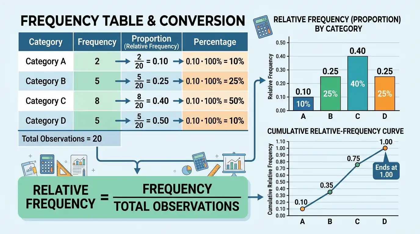
Relative frequency is the proportion of a data set represented by a particular value, category, outcome, or class interval, calculated by dividing that outcome’s frequency by the total number of observations. If an event occurs 18 times in a sample containing 60 observations, its relative frequency is 18/60 = 0.30, meaning the event accounts for 30% of the observed data. Unlike raw frequency, which reports an absolute count, relative frequency places counts on a common scale from 0 to 1, making distributions with different sample sizes much easier to compare. The relative frequencies of all mutually exclusive and collectively exhaustive categories should sum to 1, apart from small rounding differences, and multiplying any relative frequency by 100 converts it to a percentage. Because relative frequency represents an observed proportion, it also provides an important connection between descriptive data summaries and empirical probability, although an observed relative frequency should not automatically be treated as the exact underlying population probability.
Within descriptive statistics and the broader Statistics & Probability framework, relative frequency is fundamental to tables, distributions, percentages, empirical probabilities, and graphical summaries. It allows an analyst to move from the question “How many observations fall here?” to the more comparable question “What share of the total falls here?”
What Is Relative Frequency?
Relative frequency describes the fraction of all observations belonging to a particular outcome.
Suppose a data set contains:
n = 50
observations, and the value 4 occurs:
f = 15
times.
Then:
Relative frequency = 15/50
= 0.30
Therefore, the value 4 represents:
30%
of the data.
The count 15 is the frequency, while 0.30 is the relative frequency.
Relative Frequency Formula
The basic formula is:
Relative frequency = Frequency / Total number of observations
Using symbols:
rᵢ = fᵢ/n
where:
- rᵢ = relative frequency of outcome i
- fᵢ = frequency of outcome i
- n = total number of observations
If relative frequency is expressed as a percentage:
Relative frequency percentage = (fᵢ/n) × 100%
The proportion and percentage contain the same information on different numerical scales.
Simple Relative Frequency Example
Suppose a survey of:
80 people
finds that:
20
choose Option A.
Then:
r_A = 20/80
= 0.25
As a percentage:
0.25 × 100%
= 25%
Therefore:
Relative frequency of Option A = 0.25 = 25%
This means one quarter of the observed sample selected Option A.
Relative Frequency Table
Suppose 40 observations fall into four categories:
| Category | Frequency |
|---|---|
| A | 6 |
| B | 10 |
| C | 16 |
| D | 8 |
Check the total:
n = 6 + 10 + 16 + 8
= 40
Now divide every frequency by 40.
For A:
6/40 = 0.15
For B:
10/40 = 0.25
For C:
16/40 = 0.40
For D:
8/40 = 0.20
The relative-frequency table becomes:
| Category | Frequency | Relative Frequency | Percentage |
|---|---|---|---|
| A | 6 | 0.15 | 15% |
| B | 10 | 0.25 | 25% |
| C | 16 | 0.40 | 40% |
| D | 8 | 0.20 | 20% |
The largest observed share belongs to:
Category C.
Relative Frequencies Should Sum to 1
If the categories include every observation exactly once, then:
Σfᵢ = n.
Therefore:
Σrᵢ = Σ(fᵢ/n)
= (1/n)Σfᵢ
= n/n
= 1.
For the previous example:
0.15 + 0.25 + 0.40 + 0.20
= 1.00.
In percentage form:
15% + 25% + 40% + 20%
= 100%.
This provides an important calculation check.
Why Relative Frequencies Sometimes Sum to 0.99 or 1.01
Rounded relative frequencies may not sum exactly to 1.
Suppose exact proportions are:
1/3, 1/3, 1/3.
Each is approximately:
0.3333.
If rounded to two decimals, each becomes:
0.33.
Then:
0.33 + 0.33 + 0.33
= 0.99.
The underlying exact relative frequencies still sum to 1.
The discrepancy is caused only by rounding.
For this reason, calculations should normally use unrounded values and round only the displayed results.
Relative Frequency vs Frequency
Frequency is an absolute count.
Relative frequency is a proportion of the total.
Suppose:
Group A contains 100 observations
and an event occurs:
20 times.
Its frequency is:
20
and relative frequency is:
20/100 = 0.20.
Now suppose Group B contains:
1,000 observations
and the same event occurs:
150 times.
Its frequency is much larger:
150
but its relative frequency is:
150/1000
= 0.15.
Thus, the event occurs more times in absolute terms in Group B but represents a larger share of the data in Group A.
Why Relative Frequency Helps Compare Different Sample Sizes
Raw counts can be misleading when groups differ greatly in size.
Suppose Store A receives:
500 customer visits
and records:
50 returns.
Store B receives:
2,000 visits
and records:
120 returns.
Store B has more returns in absolute terms:
120 > 50.
However, relative frequencies are:
Store A = 50/500 = 0.10 = 10%
Store B = 120/2000 = 0.06 = 6%.
Relative to customer volume, returns occur more frequently at Store A.
Relative frequency therefore separates scale from proportion.
Converting Frequency to Relative Frequency
If frequency and total sample size are known:
r = f/n.
Suppose:
f = 27
n = 90.
Then:
r = 27/90
= 0.30.
Therefore:
Relative frequency = 0.30
or:
30%.
This conversion is direct because every count is standardized by the same denominator.
Converting Relative Frequency Back to Frequency
If relative frequency and total number of observations are known:
f = rn.
Suppose:
r = 0.35
and:
n = 200.
Then:
f = 0.35(200)
= 70.
Therefore:
Frequency = 70.
This relationship assumes the displayed relative frequency is sufficiently precise to reconstruct an integer frequency.
If the proportion has been heavily rounded, the original count may not be uniquely recoverable.
Example With Rounded Relative Frequency
Suppose:
n = 37
and a relative frequency is displayed as:
0.19.
Multiplying gives:
37(0.19)
= 7.03.
A frequency cannot be:
7.03 observations.
The likely original frequency may have been:
7
because:
7/37 ≈ 0.18919
which rounds to:
0.19.
This example shows why rounded relative frequencies can lose enough precision to prevent exact reconstruction.
Relative Frequency as a Percentage
To convert a relative frequency into a percentage:
Percentage = Relative frequency × 100%
If:
r = 0.42
then:
0.42 × 100%
= 42%.
Conversely:
Relative frequency = Percentage/100.
For:
17%
we obtain:
r = 17/100
= 0.17.
Proportions and percentages are simply alternative representations of the same observed share.
Relative Frequency With Decimal Percentages
Suppose:
13
of:
48
observations belong to one category.
Then:
r = 13/48
≈ 0.270833.
As a percentage:
27.0833%.
A sensible report might round this to:
27.1%.
The exact level of rounding should reflect the precision needed and should remain consistent across the table.
Relative Frequency Distribution
A relative frequency distribution lists every value or class alongside its proportion of the total.
Suppose numerical observations produce:
| Value | Frequency | Relative Frequency |
|---|---|---|
| 1 | 5 | 0.10 |
| 2 | 15 | 0.30 |
| 3 | 20 | 0.40 |
| 4 | 10 | 0.20 |
The table immediately shows that:
Value 3
accounts for:
40%
of all observations.
Unlike a frequency-only table, the same distribution can be compared directly with another sample containing a different number of observations.
Relative Frequency for Grouped Data
For grouped numerical data, each class has:
rᵢ = fᵢ/n.
Suppose:
| Interval | Frequency |
|---|---|
| 0–10 | 8 |
| 10–20 | 12 |
| 20–30 | 20 |
| 30–40 | 10 |
Total:
n = 50.
Relative frequencies are:
8/50 = 0.16
12/50 = 0.24
20/50 = 0.40
10/50 = 0.20.
Therefore:
| Interval | Relative Frequency |
|---|---|
| 0–10 | 0.16 |
| 10–20 | 0.24 |
| 20–30 | 0.40 |
| 30–40 | 0.20 |
The class:
20–30
contains 40% of the observations.
Relative Frequency and Unequal Class Widths
Relative frequency tells how much of the sample belongs to a class, regardless of the class width.
Suppose:
0–10 contains 20%
and:
10–30 contains 30%.
The second interval contains a larger proportion overall, but it is also twice as wide.
If the goal is to compare concentration per unit of measurement in a histogram with unequal bin widths, relative-frequency density is more appropriate:
Relative frequency density = Relative frequency / Class width
The distinction matters because histogram area, not necessarily bar height, should represent relative frequency when widths differ.
Relative Frequency Density Example
Suppose:
Class A: width = 10, relative frequency = 0.20
Class B: width = 20, relative frequency = 0.30.
Density for A:
0.20/10
= 0.020.
Density for B:
0.30/20
= 0.015.
Although Class B contains a larger total share, Class A has greater concentration per unit of horizontal scale.
This is why unequal-width histograms should not compare raw relative-frequency heights directly.
Cumulative Relative Frequency
Cumulative relative frequency is the running total of relative frequencies up to a particular value or class.
Suppose:
| Class | Relative Frequency |
|---|---|
| 0–10 | 0.10 |
| 10–20 | 0.25 |
| 20–30 | 0.40 |
| 30–40 | 0.25 |
Cumulative values are:
0.10
0.10 + 0.25 = 0.35
0.35 + 0.40 = 0.75
0.75 + 0.25 = 1.00.
Therefore:
| Class | Relative Frequency | Cumulative Relative Frequency |
|---|---|---|
| 0–10 | 0.10 | 0.10 |
| 10–20 | 0.25 | 0.35 |
| 20–30 | 0.40 | 0.75 |
| 30–40 | 0.25 | 1.00 |
The last cumulative value should reach:
1
apart from rounding.
Cumulative Relative Frequency Formula
If:
Fᵢ
is cumulative frequency through class i, then:
Cumulative relative frequency = Fᵢ/n.
It can also be found by adding ordinary relative frequencies:
Cᵢ = r₁ + r₂ + … + rᵢ.
Both methods give the same result.
For example, if:
75
of:
100
observations are at or below a particular class boundary:
C = 75/100
= 0.75.
Thus:
75%
of observations lie at or below that point.
Relative Frequency and Percentiles
Cumulative relative frequency helps locate approximate percentile positions.
Suppose cumulative relative frequency reaches:
0.25
near one value.
That location corresponds approximately to the:
25th percentile.
Likewise:
0.50
corresponds to the median region, while:
0.75
corresponds to the third-quartile region.
For grouped data, exact percentile values may require interpolation because the cumulative table identifies the class containing the desired percentile rather than the precise raw observation.
Relative Frequency and Probability
Relative frequency is often interpreted as an empirical probability.
Suppose an event occurs:
240
times during:
1,000
observed trials.
Its empirical relative frequency is:
240/1000
= 0.24.
One can describe:
0.24
as the observed proportion of trials in which the event occurred.
However, this does not prove that the true probability of the event is exactly:
0.24.
Sampling variability causes observed proportions to fluctuate.
Relative Frequency vs Theoretical Probability
Theoretical probability comes from a probability model.
Relative frequency comes from observed data.
For a fair six-sided die, theoretical probability of rolling a 6 is:
P(6) = 1/6
≈ 0.1667.
Suppose 60 actual rolls produce:
8 sixes.
Observed relative frequency is:
8/60
≈ 0.1333.
The two values differ.
That difference does not automatically show the die is unfair; random variation can produce discrepancies in finite samples.
Relative Frequency in Repeated Trials
Under suitable repeated-trial conditions, observed relative frequency tends to become more stable as the number of trials increases.
If an event has fixed probability:
p
and trials satisfy the assumptions required for the usual law of large numbers, then:
Relative frequency → p
as the number of observations becomes very large.
This convergence is a foundational connection between empirical frequency and probability.
It does not mean every larger sample must be closer than every smaller sample.
Random fluctuations remain possible.
Coin-Toss Example
For a fair coin:
P(Heads) = 0.5.
Suppose the first 10 tosses produce:
7 heads.
Relative frequency:
7/10
= 0.70.
After 1,000 tosses, suppose there are:
507 heads.
Relative frequency:
507/1000
= 0.507.
The larger sample happens to lie much closer to the theoretical 0.5 probability.
This illustrates the tendency toward long-run stabilization without requiring exact equality at any finite n.
Relative Frequency as a Sample Proportion
For a binary outcome, relative frequency is also called the sample proportion.
If:
x = number of successes
and:
n = total trials,
then:
p̂ = x/n.
Thus:
p̂
is simply the relative frequency of the success outcome.
For:
x = 84
n = 120,
we obtain:
p̂ = 84/120
= 0.70.
The observed success relative frequency is:
70%.
Sampling Variability of a Relative Frequency
If observations arise from independent Bernoulli trials with probability p, the sample proportion p̂ has:
E(p̂) = p
and:
Var(p̂) = p(1 − p)/n.
Therefore, its standard error is:
SE(p̂) = √[p(1 − p)/n].
This explains mathematically why relative frequencies tend to become more stable as n increases.
The denominator n reduces the sampling variance.
The formula belongs to a specific probability model and should not be assumed for arbitrary dependent or complex samples.
Relative Frequency of the Complement
If an event A has relative frequency:
r(A),
and every observation belongs either to A or not A, then:
r(not A) = 1 − r(A).
Suppose:
r(A) = 0.37.
Then:
r(not A) = 1 − 0.37
= 0.63.
In percentage terms:
37% + 63% = 100%.
This is the empirical counterpart of the complement rule in probability.
Combining Mutually Exclusive Categories
If categories A and B do not overlap, their combined relative frequency is:
r(A or B) = r(A) + r(B).
Suppose:
r(A) = 0.20
and:
r(B) = 0.35.
Then:
r(A or B) = 0.55.
Therefore:
55%
of observations belong to either A or B.
This simple addition works only when the categories are mutually exclusive for the counting scheme being used.
Relative Frequency and the Empirical Distribution
A relative-frequency table can be viewed as an empirical distribution.
For discrete values xᵢ:
Empirical probability at xᵢ = fᵢ/n.
For example:
| x | Relative Frequency |
|---|---|
| 1 | 0.20 |
| 2 | 0.50 |
| 3 | 0.30 |
behaves mathematically like a probability mass distribution because:
0.20 + 0.50 + 0.30 = 1.
This perspective makes it possible to calculate empirical means and other descriptive quantities using relative frequencies as weights.
Mean From Relative Frequencies
If numerical values xᵢ have relative frequencies rᵢ, the arithmetic mean can be calculated as:
x̄ = Σrᵢxᵢ
provided the relative frequencies represent the full sample distribution and sum to 1.
Suppose:
| x | Relative Frequency |
|---|---|
| 1 | 0.20 |
| 2 | 0.50 |
| 3 | 0.30 |
Then:
x̄ = 1(0.20) + 2(0.50) + 3(0.30)
= 0.20 + 1.00 + 0.90
= 2.10.
The relative frequencies act as empirical weights.
Population Variance From Relative Frequencies
When the distribution represents an entire finite population, population variance can be calculated directly from relative frequencies:
μ = Σrᵢxᵢ
and:
σ² = Σrᵢ(xᵢ − μ)².
Suppose:
| x | Relative Frequency |
|---|---|
| 1 | 0.25 |
| 2 | 0.50 |
| 3 | 0.25 |
The mean is:
μ = 2.
Variance is:
σ² = 0.25(1 − 2)² + 0.50(2 − 2)² + 0.25(3 − 2)²
= 0.25 + 0 + 0.25
= 0.50.
Thus, relative frequencies can encode all weighting needed for the population calculation.
Sample Variance and Relative Frequencies
For sample data, sample variance uses the sample mean and typically divides the squared-deviation total by:
n − 1.
If exact frequencies are known:
s² = Σfᵢ(xᵢ − x̄)²/(n − 1).
Since:
fᵢ = nrᵢ,
the same information can be written using relative frequencies, provided:
n
is also known.
Relative frequencies alone may not contain enough information to reproduce an unbiased sample variance because the n − 1 correction depends explicitly on sample size.
Why Sample Size Matters When Using Relative Frequencies
Consider two data sets with the identical relative-frequency distribution:
50% at 0
50% at 10.
One sample contains:
n = 10.
Another contains:
n = 1,000.
Their empirical weighted distribution shape is identical, but the usual unbiased sample-variance calculation contains different:
n/(n − 1)
corrections.
For large n the difference becomes tiny, but mathematically the sample sizes still matter.
A relative-frequency table is therefore not always sufficient for every inferential calculation unless n is also available.
Relative Frequency and Range
The range depends only on the smallest and largest observed values, whereas relative frequency tells how much data occupy each value or interval.
Suppose:
Minimum = 0
Maximum = 100.
The range is:
However, relative frequencies might show that:
99%
of observations lie between 40 and 60 and only one observation appears near each endpoint.
Another data set can have the same range but distribute observations evenly across the entire span.
Relative frequencies expose this internal structure.
Relative Frequency and Outlier Detection
Outlier detection can benefit from relative-frequency information because sparse tail regions become easy to identify.
Suppose one upper interval contains:
0.5%
of observations
while central intervals contain:
20% to 30%
each.
The low tail frequency may indicate unusual observations worth investigating.
However, low relative frequency alone does not make an observation an outlier.
Rare categories and legitimate extreme values can occur naturally.
A distance- or model-based criterion is usually needed for formal outlier classification.
Relative Frequency and Skewness
Skewness describes asymmetry, while relative frequency describes the proportion of observations occupying particular locations.
A relative-frequency distribution can visually reveal why skewness exists.
For a right-skewed variable, most relative frequency may lie in lower or middle intervals while progressively smaller proportions extend far into an upper tail.
In a left-skewed distribution, the thin tail extends toward lower values.
Relative frequency supplies the distributional mass pattern, while skewness summarizes asymmetry numerically.
Relative Frequency Does Not Measure Distance
Suppose:
Category A has relative frequency 0.20
and:
Category B has relative frequency 0.40.
This means B occurs twice as often proportionally.
It does not mean B is:
twice as far
from anything.
Relative frequency measures proportion, not numerical distance.
This distinction is especially important when categories are nominal and have no meaningful numerical spacing.
Relative Frequency for Categorical Data
Relative frequency is naturally suited to nominal categories.
Suppose preferred colors are:
| Color | Frequency |
|---|---|
| Red | 15 |
| Blue | 25 |
| Green | 10 |
Total:
n = 50.
Relative frequencies are:
Red = 15/50 = 0.30
Blue = 25/50 = 0.50
Green = 10/50 = 0.20.
No numerical ordering of colors is required.
The statistic simply measures each category’s share of the sample.
Relative Frequency for Ordinal Data
Ordinal categories can also use relative frequencies.
Suppose ratings are:
| Rating | Relative Frequency |
|---|---|
| Poor | 0.05 |
| Fair | 0.15 |
| Good | 0.40 |
| Very Good | 0.30 |
| Excellent | 0.10 |
The proportions show the distribution across ordered responses.
Because the categories have order, cumulative relative frequencies are also meaningful.
For example, the proportion at or below Good is:
0.05 + 0.15 + 0.40
= 0.60.
Thus:
60%
of responses are Good or lower.
Relative Frequency for Continuous Data
Continuous measurements usually do not repeat at exactly the same value when recorded with high precision.
Therefore, relative frequencies are often calculated for intervals.
For example:
0 ≤ x < 10
might contain:
12%
of observations.
The next interval:
10 ≤ x < 20
might contain:
28%.
Grouping produces an approximate distributional summary while preserving the proportion of observations within each interval exactly if the class counts are known.
Choosing Classes
Class definitions affect how a grouped relative-frequency distribution looks.
Suppose many observations lie between:
19 and 21.
Bins:
10–20
and:
20–30
split that concentration across two classes.
A different binning scheme:
15–25
might place most of it together.
The underlying observations have not changed.
Only their grouping has.
Therefore, small graphical differences should not be overinterpreted when they are sensitive to arbitrary class boundaries.
Relative Frequency and Histograms
For equal-width classes, relative-frequency histograms can use:
bar height = class relative frequency.
The resulting shape is identical to the raw-frequency histogram apart from vertical scaling because every count is divided by the same n.
For unequal-width bins, however, bar area should represent relative frequency, which requires:
Height = Relative frequency / Class width.
This distinction preserves the correct visual proportions.
Frequency Histogram vs Relative-Frequency Histogram
Suppose one class has:
f = 20
in a sample of:
n = 100.
Its relative frequency is:
0.20.
In a raw-frequency histogram the bar may have height:
In a relative-frequency histogram it may have height:
0.20.
If all class widths are equal, every bar is simply scaled by:
1/n.
Therefore, both histograms have the same overall shape.
The vertical-axis interpretation is what changes.
Comparing Two Relative-Frequency Distributions
Suppose Sample A contains:
n = 100
and Sample B:
n = 10,000.
Using raw counts makes Sample B’s bars much taller even if the distributions are proportionally identical.
Relative frequencies place both on a common scale.
If 30% of each sample occupies the same interval:
Sample A frequency = 30
Sample B frequency = 3,000
but:
Relative frequency = 0.30
for both.
This allows direct comparison of distribution shape rather than sample size.
Weighted Relative Frequency
Some data sets assign weights to observations.
A weighted relative frequency for category A can be calculated as:
Weighted relative frequency = Sum of weights in A / Sum of all weights
Suppose three observations in A have weights:
2, 3, 5
and total weight across the data is:
Then:
Weighted r_A = (2 + 3 + 5)/25
= 10/25
= 0.40.
This means category A represents 40% of the weighted total, even if its unweighted observation count represents a different percentage.
Weighted vs Unweighted Relative Frequency
Suppose 10 respondents are surveyed.
Only:
2
belong to Category A, so the unweighted relative frequency is:
2/10
= 0.20.
If those respondents receive large survey weights and collectively represent:
35%
of the weighted population estimate, then:
Weighted relative frequency = 0.35.
Neither result is automatically wrong.
They answer different questions:
sample composition
versus:
weighted estimated composition.
The weighting method should be stated clearly.
Relative Frequency and Missing Data
The denominator is critically important when observations are missing.
Suppose 100 people are surveyed:
Yes = 45
No = 35
Missing = 20.
If relative frequencies are based on all selected records:
Yes = 45/100 = 45%.
If the analysis excludes missing responses and uses only 80 valid answers:
Yes = 45/80
= 56.25%.
Both calculations are mathematically correct but answer different questions.
The denominator should therefore be defined explicitly.
Valid Percent
When missing observations are excluded from a categorical percentage calculation, the resulting proportion is sometimes called:
valid percent.
Using the previous example:
Valid n = 45 + 35
= 80.
Therefore:
Yes valid percent = 45/80 × 100%
= 56.25%.
Reporting both overall and valid percentages can make missingness transparent.
The choice should depend on what population of observations the percentage is intended to describe.
Relative Frequency of Missing Values
Missingness can itself be summarized.
If:
20
of:
100
records are missing:
Missing relative frequency = 20/100
= 0.20.
Thus:
20%
of records lack a valid response.
This is useful because missing-data prevalence can materially affect interpretation even when missing values are excluded from substantive category percentages.
Zero Relative Frequency
A possible outcome can have relative frequency:
0
if it does not occur in the observed sample.
For example, a six-sided die rolled 10 times might never produce a 6.
Then:
Observed relative frequency of 6 = 0/10
= 0.
This does not prove:
P(6) = 0.
It only means the outcome was not observed in that finite sample.
Relative Frequency of One
Relative frequency equals:
1
when every observation belongs to the same category.
Suppose all 40 respondents select:
Option A.
Then:
r_A = 40/40
= 1.
As a percentage:
100%.
All other mutually exclusive alternatives have observed relative frequency:
Relative Frequency Is Between 0 and 1
Because:
0 ≤ fᵢ ≤ n,
dividing by positive n gives:
0 ≤ fᵢ/n ≤ 1.
Therefore:
0 ≤ rᵢ ≤ 1.
A calculated ordinary relative frequency such as:
1.25
or:
−0.10
indicates an error in the count, denominator, or definition.
Weighted methods can also be constrained to this range when nonnegative weights and mutually exclusive categories are used.
Percent Relative Frequency Is Between 0% and 100%
Multiplying the proportion range by 100 gives:
0% ≤ Relative frequency percentage ≤ 100%.
If a single mutually exclusive category is reported as:
135%
there is a problem.
However, percentages can legitimately sum above 100% in multiple-response questions where one observation may belong to several categories.
The counting framework must therefore be understood before using the sum-to-100 rule.
Multiple-Response Data
Suppose respondents can select several hobbies.
A person may choose:
Reading
and:
Sports.
If category percentages are calculated as:
Number selecting category / Number of respondents,
then percentages across hobbies can sum to more than:
100%.
This does not violate arithmetic because the categories are not mutually exclusive.
The rule:
Σ relative frequencies = 1
applies when every observation is allocated exactly once across the categories being summed.
Joint Relative Frequency
For two categorical variables, joint relative frequency measures the proportion belonging to a particular combination.
Suppose:
30
of:
200
customers are both:
New customers
and:
Premium-plan users.
Then:
Joint relative frequency = 30/200
= 0.15.
Therefore:
15%
of all observed customers fall into that combination.
A two-way table can display joint relative frequencies across all category pairs.
Marginal Relative Frequency
In a two-way table, marginal relative frequency summarizes one variable without conditioning on the other.
Suppose:
80
of:
200
customers use the Premium plan.
Then:
Premium marginal relative frequency = 80/200
= 0.40.
It is called marginal because totals are commonly displayed at the table margins.
Marginal and joint frequencies answer different questions.
Conditional Relative Frequency
Conditional relative frequency changes the denominator to a subgroup.
Suppose among:
80 Premium users,
there are:
30 new customers.
Then:
Conditional relative frequency = 30/80
= 0.375.
Therefore:
37.5%
of Premium users are new customers.
This differs from the joint relative frequency:
30/200 = 15%.
Changing the denominator changes the interpretation.
Denominator Choice Is Fundamental
Many relative-frequency errors are denominator errors rather than arithmetic errors.
Suppose:
40 women
and:
60 men
are surveyed.
If:
20 women
choose Option A, then:
20/100 = 20%
is the proportion of all respondents who are women choosing A.
But:
20/40 = 50%
is the proportion of women who choose A.
Both are valid relative frequencies.
The intended reference group determines which denominator is correct.
Relative Frequency and Rates
Relative frequency is sometimes casually called a rate, but not every rate is a relative frequency.
For example:
20 defects / 100 items
is a proportion:
0.20.
But:
20 accidents / 1,000 vehicle-hours
is an incidence rate based on exposure rather than a fraction of observations belonging to one category.
The units and denominator structure matter.
Relative frequencies are dimensionless proportions, whereas exposure rates can have units such as events per hour.
Relative Frequency and Ratios
A relative frequency:
fᵢ/n
compares one category with the total.
A ratio might compare two categories directly:
f_A/f_B.
Suppose:
A = 30
B = 20
Total = 100.
Relative frequencies are:
A = 0.30
B = 0.20.
The ratio A:B is:
30/20
= 1.5.
A relative frequency and a category-to-category ratio answer different questions.
Relative Frequency and Proportions
In many elementary contexts, “relative frequency” and “observed proportion” are mathematically equivalent:
Proportion = Count of interest / Total count.
The terminology often depends on context.
A frequency table emphasizes:
relative frequency.
A survey estimate may emphasize:
sample proportion.
A probability experiment may use:
empirical probability.
The underlying calculation can be identical.
Relative Frequency and Sample Composition
Relative frequency provides a compact description of sample composition.
Suppose a sample consists of:
20% Group A
30% Group B
50% Group C.
These values show immediately how observations are distributed across groups.
However, they do not establish that the wider target population has the same proportions.
If sampling is biased, sample relative frequencies can differ systematically from population proportions.
Sampling Bias
Suppose an online survey produces:
70%
support for an option.
The relative frequency of support in the respondents is indeed:
0.70.
However, if participation is voluntary and respondents differ systematically from nonrespondents, 0.70 may be a biased estimate of the population proportion.
Relative frequency accurately summarizes the observed data.
Generalizing it requires an appropriate sampling design and inferential assumptions.
Relative Frequency and Random Sampling
Under representative random sampling, sample relative frequencies can estimate population proportions.
Suppose a population contains an unknown proportion p of a category.
A random sample produces:
p̂ = f/n.
The sample relative frequency:
p̂
is then used as an estimator of:
p.
Its reliability depends on sample size and sampling design.
The descriptive calculation itself remains the same regardless of how the sample was collected.
Larger n Does Not Guarantee an Unbiased Relative Frequency
Increasing sample size reduces random sampling variability under suitable conditions, but it does not automatically remove systematic bias.
Suppose a survey method consistently excludes one subgroup.
Increasing:
n = 1,000
to:
n = 1,000,000
can make the observed relative frequencies extremely stable while still representing the wrong population composition.
Precision and representativeness are different properties.
A large denominator is not a substitute for sound sampling.
Relative Frequency and Rounding
Suppose frequencies are:
1, 1, 1
with:
n = 3.
Exact relative frequencies are:
0.333333…
for each category.
If rounded to:
0.33
the displayed total becomes:
0.99.
If displayed as percentages rounded to whole numbers:
33% + 33% + 33%
= 99%.
This is a display issue rather than a substantive problem.
Keeping more decimal places or adjusting presentation can reduce apparent discrepancies.
Common Relative Frequency Mistakes
A common mistake is dividing a category’s frequency by the wrong denominator. The denominator should represent the full reference group for the relative frequency being reported.
Another error is multiplying by 100 and then still describing the result as a decimal proportion. A relative frequency of 0.25 is equivalent to 25%, not 0.25%.
Analysts also sometimes expect rounded categories to sum exactly to 1 or 100%, even though rounding can introduce small discrepancies.
Another mistake is treating an observed relative frequency as though it were automatically the exact theoretical probability.
For grouped histograms with unequal class widths, using relative frequency directly as bar height can also misrepresent concentration; relative-frequency density is required when area should encode proportion.
Missing values, overlapping categories, and survey weights can all alter the correct denominator, so those conventions should be specified rather than assumed.
Finally, a category with low relative frequency is not automatically an outlier or error.
How to Calculate Relative Frequency Step by Step
Begin by counting the number of valid observations in the reference group:
n.
Count how many belong to the outcome or class of interest:
f.
Calculate:
r = f/n.
If a percentage is desired:
Percentage = 100r.
Repeat for every mutually exclusive category and check:
Σr ≈ 1
or:
ΣPercentage ≈ 100%.
If the total differs materially rather than by rounding, check for missing observations, overlapping categories, omitted categories, or denominator errors.
Full Worked Example
Suppose a class of 60 students receives the following grades:
| Grade | Frequency |
|---|---|
| A | 9 |
| B | 18 |
| C | 21 |
| D | 9 |
| F | 3 |
Step 1: Verify Total Frequency
n = 9 + 18 + 21 + 9 + 3
= 60
Step 2: Calculate Each Relative Frequency
For A:
9/60
= 0.15
For B:
18/60
= 0.30
For C:
21/60
= 0.35
For D:
9/60
= 0.15
For F:
3/60
= 0.05
Build the Final Table
| Grade | Frequency | Relative Frequency | Percentage |
|---|---|---|---|
| A | 9 | 0.15 | 15% |
| B | 18 | 0.30 | 30% |
| C | 21 | 0.35 | 35% |
| D | 9 | 0.15 | 15% |
| F | 3 | 0.05 | 5% |
Check:
0.15 + 0.30 + 0.35 + 0.15 + 0.05
= 1.00.
Therefore, the distribution is internally consistent.
The most common observed grade is C, representing:
35%
of the class.
Cumulative Relative Frequency for the Grade Example
If grades are treated in ordered sequence from A through F, cumulative relative frequencies are:
For A:
0.15
Through B:
0.15 + 0.30
= 0.45
Through C:
0.45 + 0.35
= 0.80
Through D:
0.80 + 0.15
= 0.95
Through F:
1.00.
Whether cumulative interpretation is substantively useful depends on the chosen ordering and the question being asked.
Full Grouped Numerical Example
Suppose 100 observations are grouped as:
| Interval | Frequency |
|---|---|
| 0–20 | 10 |
| 20–40 | 25 |
| 40–60 | 40 |
| 60–80 | 20 |
| 80–100 | 5 |
Because:
n = 100,
the relative frequencies are immediately:
0.10, 0.25, 0.40, 0.20, 0.05.
Therefore:
| Interval | Frequency | Relative Frequency |
|---|---|---|
| 0–20 | 10 | 0.10 |
| 20–40 | 25 | 0.25 |
| 40–60 | 40 | 0.40 |
| 60–80 | 20 | 0.20 |
| 80–100 | 5 | 0.05 |
The central:
40–60
interval contains the largest observed share:
40%.
Compare Samples of Different Sizes
Suppose another sample contains:
n = 1,000
with frequencies:
90, 260, 410, 190, 50
across the same intervals.
Its relative frequencies are:
0.09, 0.26, 0.41, 0.19, 0.05.
Although every raw frequency is much larger than in the 100-observation sample, the relative-frequency patterns are very similar.
This is exactly why proportion-based distributions are useful for comparing groups of unequal size.
How to Report Relative Frequency
A clear statement includes the count, denominator, and proportion when practical.
For example:
“Twenty-one of 60 students received a C, giving a relative frequency of 0.35, or 35%.”
For grouped data:
“The 40–60 interval contained 40 of 100 observations, corresponding to a relative frequency of 0.40.”
Including the raw count alongside the proportion can be useful because:
40%
of 10 observations
and:
40%
of 10,000 observations
represent very different amounts of data.
When Relative Frequency Is Most Useful
Relative frequency is particularly useful when:
- sample sizes differ;
- percentages are more interpretable than counts;
- probability-like empirical distributions are needed;
- categorical composition matters;
- grouped numerical distributions are being compared;
- cumulative proportions are useful;
- data must be standardized to a common scale.
It is one of the simplest ways to make frequency information comparable across groups.
When Raw Frequency Is Still Important
Relative frequency should not completely replace the original count.
Suppose:
50%
of Sample A
and:
50%
of Sample B
belong to one category.
If:
n_A = 4
and:
n_B = 100,000,
the evidential strength and operational magnitude are very different.
Reporting:
frequency + relative frequency
provides both scale and proportion.
A percentage without its denominator can hide important context.
Frequently Asked Questions About Relative Frequency
What is relative frequency?
Relative frequency is the proportion of all observations belonging to a particular value, category, outcome, or interval.
What is the formula?
Relative frequency = Frequency / Total observations
What is the symbolic formula?
rᵢ = fᵢ/n
What does fᵢ mean?
The frequency of outcome i.
What does n mean?
The total number of observations in the relevant denominator.
How do you convert relative frequency to a percentage?
Percentage = Relative frequency × 100%
What is the relative frequency of 20 out of 80?
20/80 = 0.25 = 25%.
What is the relative frequency of 7 out of 50?
7/50 = 0.14 = 14%.
What should relative frequencies sum to?
For mutually exclusive categories covering every observation:
What should percentage relative frequencies sum to?
100%.
Why might they sum to 99% or 101%?
Rounding.
Can relative frequency be greater than 1?
Not for an ordinary single category defined as a subset of the denominator.
Can relative frequency be negative?
No.
Can relative frequency equal zero?
Yes, if the outcome does not occur.
Does zero relative frequency mean the event is impossible?
No. It means the event was not observed in that sample.
Can relative frequency equal one?
Yes, if every observation belongs to that category.
Is relative frequency the same as frequency?
No. Frequency is a count; relative frequency is a proportion.
Is relative frequency the same as percentage?
A percentage is the relative frequency multiplied by 100.
Is relative frequency the same as probability?
Not exactly. Relative frequency is observed empirically, while theoretical probability belongs to a probability model.
Can relative frequency estimate probability?
Yes, under appropriate sampling or repeated-trial conditions.
What happens to relative frequency as trials increase?
Under suitable conditions, it tends to stabilize around the underlying event probability.
Is relative frequency the same as a sample proportion?
For a binary event, yes:
p̂ = x/n.
Can relative frequency be used for categorical data?
Yes.
Can it be used for nominal data?
Yes.
Can it be used for ordinal data?
Yes.
Can it be used for continuous data?
Yes, usually by grouping observations into intervals.
What is a relative frequency distribution?
A table or representation showing the proportion associated with each value or class.
What is cumulative relative frequency?
The running sum of relative frequencies through an ordered value or class.
What should the last cumulative relative frequency equal?
1
or:
100%.
How do you calculate cumulative relative frequency?
Either sum preceding relative frequencies or divide cumulative frequency by n.
Can relative frequency help locate percentiles?
Yes, cumulative relative frequencies can identify approximate percentile locations.
What is relative-frequency density?
Relative frequency / Class width.
When is relative-frequency density important?
When histogram bins have unequal widths and bar area should represent relative frequency.
Why not use ordinary relative-frequency height for unequal bins?
Because wider bins would receive excessive visual area relative to their concentration.
Can frequency be recovered from relative frequency?
Yes, if n is known and the relative frequency has sufficient precision:
f = rn.
Can rounded relative frequencies prevent exact recovery?
Yes.
Why are relative frequencies useful for samples of different sizes?
They place counts on the same 0-to-1 or 0%-to-100% scale.
Can two samples have very different frequencies but identical relative frequencies?
Yes.
Does the larger frequency always represent the larger relative frequency?
No.
What is weighted relative frequency?
Sum of category weights / Sum of all weights.
Is weighted relative frequency the same as ordinary relative frequency?
Not necessarily.
Can missing values change relative frequency?
Yes, because including or excluding them changes the denominator.
What is valid percent?
A percentage calculated among observations with valid nonmissing responses.
Can missingness itself have a relative frequency?
Yes.
Can category percentages add above 100%?
Yes, if observations can select multiple categories and therefore belong to more than one category.
When must they sum to 100%?
When the categories are mutually exclusive and collectively exhaustive.
What is joint relative frequency?
The proportion of all observations belonging to a specific combination of categories.
What is marginal relative frequency?
The overall proportion belonging to one category regardless of another variable.
What is conditional relative frequency?
A proportion calculated within a specified subgroup.
Why is the denominator so important?
Because changing the denominator changes the population or subgroup being described.
Is relative frequency a measure of spread?
No.
Is it a measure of distance?
No.
Can relative frequencies be used to calculate a mean?
Yes, for numerical values:
x̄ = Σrᵢxᵢ.
Can relative frequencies be used to calculate population variance?
Yes:
σ² = Σrᵢ(xᵢ − μ)²
when they describe the full population distribution.
Can they be used for sample variance?
Yes, when enough information—including sample size—is available.
Does relative frequency identify skewness directly?
No, but the pattern of relative frequencies across ordered intervals helps reveal asymmetric distribution shape.
Does a low relative frequency mean an observation is an outlier?
No.
Can relative frequency help investigate outliers?
Yes, by showing how much data occupy sparse tail regions, but a formal outlier rule requires additional criteria.
Does relative frequency tell the range?
No. Range depends only on minimum and maximum.
Can two distributions have the same range but different relative-frequency patterns?
Yes.
Does sample size affect the precision of a relative frequency?
Yes. Under suitable sampling conditions, larger samples generally produce more stable estimates of underlying population proportions.
Does a huge sample guarantee an unbiased relative frequency?
No. Systematic sampling bias can remain regardless of sample size.
Should counts be reported alongside relative frequencies?
Often yes, because the denominator and absolute amount of data provide important context.
What is the main advantage of relative frequency?
It converts counts into comparable proportions, allowing distributions with different total sizes to be interpreted on a common scale.
What is its main limitation?
A relative frequency summarizes only the observed proportion and can be misleading if the denominator, missing-data treatment, overlapping categories, sampling design, or weighting method is unclear.
What is the most important rule when calculating relative frequency?
Use the correct reference-group denominator, divide each category’s count by that total, preserve sufficient precision before rounding, and interpret the result as an observed proportion rather than automatically treating it as an exact population probability.



