
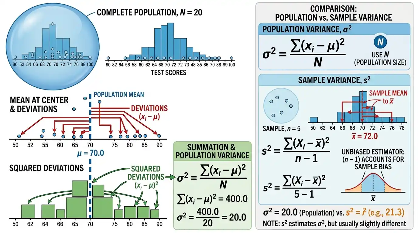
Population Variance: Definition, Formula & Example

Population variance is a measure of statistical dispersion that describes the average squared distance between every value in a defined population and that population’s arithmetic mean. For population values x₁, x₂, …, xN with population mean μ, population variance is calculated as σ² = Σ(xᵢ − μ)²/N, where every population member is included and the squared deviations are divided by the total population size N. Squaring the deviations prevents positive and negative differences from canceling while also giving greater mathematical influence to observations located farther from the mean, which makes variance fundamental to probability theory, standard deviation, statistical modeling, and many inferential procedures. Population variance differs from the familiar unbiased sample-variance estimator because there is no need to compensate for estimating an unknown population mean when the complete population itself is being summarized. Its squared units can make direct interpretation less intuitive than standard deviation, yet variance has exceptionally useful mathematical properties, including simple transformation rules, additive behavior under appropriate independence conditions, and a central role in expectations and probability distributions.
Within descriptive statistics and the broader Statistics & Probability framework, population variance answers a precise question: how much do all members of this population vary around their population mean, on average, when deviations are measured in squared units? That definition makes it important to distinguish a complete population from a sample, because using N or n − 1 in the denominator reflects different statistical objectives.
What Is Population Variance?
Population variance is the mean of the squared deviations of all population values from the population mean.
For a population containing:
x₁, x₂, …, xN
first calculate the population mean:
μ = Σxᵢ/N
Then calculate the difference between each observation and μ:
xᵢ − μ
Square every deviation:
(xᵢ − μ)²
Add those squared deviations and divide by:
N
The result is:
Population variance = σ²
Population Variance Formula
The standard formula is:
σ² = Σ(xᵢ − μ)²/N
where:
- σ² = population variance
- xᵢ = individual population value
- μ = population mean
- N = number of values in the population
- Σ = sum across all population values
The formula uses every member of the defined population.
Because the deviations are squared, population variance can never be negative.
Population Mean Formula
Population variance is calculated around the population mean:
μ = Σxᵢ/N
Suppose the population is:
2, 4, 6, 8
Then:
μ = (2 + 4 + 6 + 8)/4
= 20/4
= 5
This mean becomes the reference point for all squared deviations.
Simple Population Variance Example
Consider the complete population:
2, 4, 6, 8
The population mean is:
μ = 5
Now calculate deviations:
2 − 5 = −3
4 − 5 = −1
6 − 5 = 1
8 − 5 = 3
Square them:
9, 1, 1, 9
Their sum is:
20
Divide by:
N = 4
Therefore:
σ² = 20/4
= 5
So:
Population variance = 5
Why Deviations Are Squared
If ordinary deviations were added directly, they would cancel.
For:
−3, −1, 1, 3
the total is:
That does not mean the population has no variability.
Squaring produces:
9, 1, 1, 9
so every departure contributes positively.
The squared-deviation approach also gives greater weight to observations farther from the mean, which is both a useful mathematical feature and the reason variance is sensitive to extreme observations.
Population Variance Step by Step
To calculate population variance manually, begin by identifying the complete population and determining its arithmetic mean.
Next, subtract the mean from every value:
Deviation = xᵢ − μ
Then square each result:
Squared deviation = (xᵢ − μ)²
Add all squared deviations:
Σ(xᵢ − μ)²
Finally divide by the number of population values:
σ² = Σ(xᵢ − μ)²/N
The denominator is N because the calculation describes the population directly rather than using a sample to estimate an unknown population variance.
Worked Example With Five Values
Consider:
3, 5, 7, 9, 11
First calculate the mean:
μ = (3 + 5 + 7 + 9 + 11)/5
= 35/5
= 7
Deviations are:
−4, −2, 0, 2, 4
Squared deviations are:
16, 4, 0, 4, 16
Their sum is:
40
Therefore:
σ² = 40/5
= 8
The population variance is:
8
Population Standard Deviation
Population standard deviation is the square root of population variance:
σ = √σ²
For the previous population:
σ² = 8
Therefore:
σ = √8
≈ 2.828
The standard deviation is approximately:
2.83 units
while variance is:
8 square units.
Standard deviation is often easier to interpret because it returns to the original measurement units.
Population Variance vs Population Standard Deviation
Variance and standard deviation measure related aspects of spread.
Population variance:
σ² = average squared deviation from μ
Population standard deviation:
σ = √σ²
Variance is especially useful algebraically and theoretically.
Standard deviation is usually easier to communicate because it has the same units as the observations.
If heights are measured in centimeters:
Standard deviation → centimeters
but:
Variance → square centimeters.
Why Population Variance Has Squared Units
Suppose x is measured in:
meters.
A deviation:
x − μ
is also measured in meters.
Squaring it produces:
meters².
Averaging the squared deviations does not change that unit.
Therefore:
Population variance is measured in meters².
This squared-unit property is one reason statisticians often report standard deviation alongside variance when practical interpretation matters.
Population Variance Cannot Be Negative
Every squared deviation satisfies:
(xᵢ − μ)² ≥ 0.
Therefore:
Σ(xᵢ − μ)² ≥ 0.
Since:
N > 0,
we obtain:
σ² ≥ 0.
A negative calculated population variance therefore indicates a computational or numerical problem.
Exact mathematical variance cannot be negative.
When Population Variance Equals Zero
Population variance equals zero only when every population value is identical.
Suppose:
10, 10, 10, 10
Then:
μ = 10.
Every deviation is:
Therefore:
σ² = 0.
Conversely, if even one population value differs from the others, at least one squared deviation is positive and the variance must be greater than zero.
Population Variance With Negative Values
Negative population values cause no special difficulty.
Consider:
−4, −2, 0, 2, 4
The mean is:
μ = 0.
Squared deviations are:
16, 4, 0, 4, 16.
Sum:
Population size:
N = 5.
Therefore:
σ² = 40/5
= 8.
Variance itself remains nonnegative even when the observations are negative.
Population Variance With Decimal Values
Variance works normally with decimal observations.
Consider:
1.5, 2.5, 3.5
Population mean:
μ = (1.5 + 2.5 + 3.5)/3
= 7.5/3
= 2.5.
Deviations:
−1, 0, 1.
Squared deviations:
1, 0, 1.
Therefore:
σ² = 2/3
≈ 0.667.
The population variance is approximately:
0.67 square units.
Computational Population Variance Formula
An equivalent formula is:
σ² = Σxᵢ²/N − μ²
This is sometimes called the computational or shortcut formula.
Since:
μ = Σxᵢ/N
it can also be written:
σ² = Σxᵢ²/N − (Σxᵢ/N)²
The formula is mathematically equivalent to the deviation-based definition.
It can reduce manual work when sums of values and squared values are already available.
Deriving the Shortcut Formula
Begin with:
σ² = (1/N)Σ(xᵢ − μ)²
Expand the square:
(xᵢ − μ)² = xᵢ² − 2μxᵢ + μ²
Therefore:
σ² = (1/N)[Σxᵢ² − 2μΣxᵢ + Nμ²]
Because:
Σxᵢ = Nμ
we obtain:
σ² = Σxᵢ²/N − 2μ² + μ²
so:
σ² = Σxᵢ²/N − μ².
Shortcut Formula Example
For:
2, 4, 6, 8
calculate:
Σxᵢ² = 2² + 4² + 6² + 8²
= 4 + 16 + 36 + 64
= 120
Therefore:
Σxᵢ²/N = 120/4
= 30.
The mean is:
μ = 5.
Thus:
σ² = 30 − 5²
= 30 − 25
= 5.
This matches the direct squared-deviation calculation.
Numerical Stability of the Shortcut Formula
Although the computational identity is exact mathematically, it can be less numerically stable in finite-precision computing when values are very large but their variance is relatively small.
For example, if all observations are near:
1,000,000,000
then both:
Σx²/N
and:
μ²
can be enormous numbers whose difference is comparatively tiny.
Subtracting nearly equal large floating-point quantities can lose numerical precision.
Reliable statistical software often uses more stable algorithms rather than naïvely applying the shortcut formula.
Population Variance vs Sample Variance
Population variance describes a complete population:
σ² = Σ(xᵢ − μ)²/N
A commonly used unbiased sample variance estimator is:
s² = Σ(xᵢ − x̄)²/(n − 1)
where:
- x̄ = sample mean
- n = sample size
The denominator difference is fundamental.
Use:
N
when summarizing the complete defined population.
Use:
n − 1
when estimating an unknown population variance from a random sample under the standard unbiased sample-variance procedure.
Why Sample Variance Uses n − 1
When a population mean μ is unknown, the sample mean x̄ is estimated from the same data.
The deviations from x̄ satisfy a constraint:
Σ(xᵢ − x̄) = 0.
Only:
n − 1
of those deviations can vary independently once x̄ has been estimated.
Dividing by n would systematically underestimate population variance under the standard independent identically distributed sampling framework.
Dividing by:
n − 1
corrects that bias for the conventional sample variance estimator.
Population vs Sample Example
Suppose the observed values are:
2, 4, 6, 8.
Their mean is:
Squared-deviation sum:
If these four values are the entire population:
σ² = 20/4
= 5.
If these four values are a sample used to estimate a larger population variance:
s² = 20/(4 − 1)
= 20/3
≈ 6.667.
The same numbers produce different variance formulas because the statistical objective differs.
Is a Data Set a Sample or Population?
Population status depends on the question being asked, not merely on how many values are available.
Suppose a company records the salaries of:
all 50 employees.
If the target population is:
those exact 50 current employees,
the data constitute the complete population.
If the same 50 employees are being treated as observations from a broader process representing:
future employees,
similar companies,
or:
a larger labor market,
they function as a sample for that inferential target.
The correct denominator follows the target population.
Population Variance From a Frequency Distribution
When exact population values are summarized by frequencies, the variance can be calculated without expanding every repeated observation.
If xᵢ occurs fᵢ times:
N = Σfᵢ
Population mean:
μ = Σfᵢxᵢ/N
Population variance:
σ² = Σfᵢ(xᵢ − μ)²/N
This is mathematically identical to writing every repeated value separately.
A frequency table simply makes the calculation more efficient.
Frequency Distribution Example
Suppose:
| Value | Frequency |
|---|---|
| 1 | 2 |
| 2 | 3 |
| 4 | 1 |
Total population size:
N = 2 + 3 + 1
= 6.
Population mean:
μ = [1(2) + 2(3) + 4(1)]/6
= (2 + 6 + 4)/6
= 12/6
= 2.
Now calculate weighted squared deviations.
For x = 1:
f(x − μ)² = 2(1 − 2)²
= 2.
For x = 2:
3(2 − 2)² = 0.
For x = 4:
1(4 − 2)² = 4.
Total:
Therefore:
σ² = 6/6
= 1.
Population Variance Using Relative Frequency
A relative frequency distribution can be interpreted as population proportions when every population member is represented.
If:
pᵢ = fᵢ/N
then:
Σpᵢ = 1.
Population mean becomes:
μ = Σpᵢxᵢ
and population variance becomes:
σ² = Σpᵢ(xᵢ − μ)².
This is the same structure used for discrete probability distributions.
Relative frequency therefore provides a direct bridge between observed population counts and probability-weighted variance.
Relative Frequency Example
Using the previous population:
| Value | Relative Frequency |
|---|---|
| 1 | 2/6 |
| 2 | 3/6 |
| 4 | 1/6 |
Mean:
μ = 1(2/6) + 2(3/6) + 4(1/6)
= 2.
Variance:
σ² = (2/6)(1 − 2)² + (3/6)(2 − 2)² + (1/6)(4 − 2)²
= 2/6 + 0 + 4/6
= 6/6
= 1.
The result matches the frequency-count calculation exactly.
Population Variance for a Discrete Random Variable
If X is a discrete random variable with possible values x and probability mass function p(x), then:
μ = E(X) = Σx p(x)
and:
Var(X) = Σ(x − μ)²p(x).
The same variance can also be written:
Var(X) = E(X²) − [E(X)]².
This probability form generalizes the finite-population relative-frequency formula.
Instead of empirical frequencies, the weights are theoretical probabilities.
Expected-Value Formula
A fundamental identity is:
Var(X) = E[(X − μ)²]
where:
μ = E(X).
Expanding gives:
Var(X) = E(X²) − [E(X)]².
This identity is extremely important in probability calculations because:
E(X²)
can sometimes be easier to determine than directly averaging squared deviations.
It is the probability analogue of the computational population-variance formula.
Discrete Probability Example
Suppose X has distribution:
| x | P(X=x) |
|---|---|
| 0 | 0.25 |
| 1 | 0.50 |
| 2 | 0.25 |
Mean:
μ = 0(0.25) + 1(0.50) + 2(0.25)
= 1.
Second moment:
E(X²) = 0²(0.25) + 1²(0.50) + 2²(0.25)
= 0 + 0.50 + 1
= 1.5.
Therefore:
Var(X) = 1.5 − 1²
= 0.5.
Bernoulli Population Variance
For a Bernoulli random variable:
X = 1 with probability p
X = 0 with probability 1 − p.
The mean is:
μ = p.
Variance is:
Var(X) = p(1 − p).
For:
p = 0.5,
variance is:
0.5(0.5)
= 0.25.
This is the maximum Bernoulli variance because binary uncertainty is greatest when the two outcomes are equally likely.
Bernoulli Variance Near 0 or 1
Suppose:
p = 0.99.
Then:
Var(X) = 0.99(0.01)
= 0.0099.
The outcome is much less variable because one result occurs almost all the time.
Likewise:
p = 0.01
produces the same variance:
0.0099.
Bernoulli variance therefore reflects uncertainty rather than the numerical size of p alone.
Population Variance From Grouped Data
When only grouped intervals are available, exact population variance usually cannot be recovered because the exact individual values inside each class are unknown.
A common approximation uses class midpoints:
mᵢ = midpoint of class i.
Approximate mean:
μ ≈ Σfᵢmᵢ/N
Approximate variance:
σ² ≈ Σfᵢ(mᵢ − μ)²/N.
The result should be identified as approximate.
Grouping replaces every observation in a class with the same midpoint.
Grouped Variance Example
Suppose:
| Interval | Frequency | Midpoint |
|---|---|---|
| 0–10 | 4 | 5 |
| 10–20 | 6 | 15 |
| 20–30 | 10 | 25 |
Total:
N = 20.
Approximate mean:
μ ≈ [4(5) + 6(15) + 10(25)]/20
= 360/20
= 18.
Now calculate approximate squared deviations.
For midpoint 5:
4(5 − 18)² = 4(169) = 676.
For 15:
6(15 − 18)² = 6(9) = 54.
For 25:
10(25 − 18)² = 10(49) = 490.
Total:
1,220.
Therefore:
σ² ≈ 1220/20
= 61.
Why Grouped Population Variance Is Approximate
The midpoint method assumes every observation inside a class can be represented by its midpoint.
For the interval:
20–30,
an actual observation might be:
20.1
or:
29.9.
Both are replaced with:
Since variance depends on squared distance from the mean, these lost within-class differences can matter substantially.
Wider classes generally create greater potential approximation error.
Raw observations are preferable when exact variance matters.
Population Variance and Outliers
Population variance is highly sensitive to extreme observations because squared deviations grow rapidly.
Suppose a deviation is:
Its squared contribution is:
If a deviation is:
20,
its contribution becomes:
The second observation is ten times farther from the mean but contributes one hundred times as much before averaging.
This is why outlier detection can be important when interpreting unusually large population variance.
Extreme-Value Example
Consider the population:
1, 2, 3, 4, 5
Mean:
μ = 3.
Squared deviations:
4, 1, 0, 1, 4.
Therefore:
σ² = 10/5
= 2.
Now replace 5 with:
The new population is:
1, 2, 3, 4, 100.
Its mean becomes:
μ = 110/5
= 22.
The variance increases dramatically.
This reflects a genuine mathematical consequence of the distant observation rather than an error in the formula.
Calculate the Extreme-Value Variance
For:
1, 2, 3, 4, 100
with:
μ = 22,
deviations are:
−21, −20, −19, −18, 78.
Squared deviations:
441, 400, 361, 324, 6084.
Total:
Therefore:
σ² = 7610/5
= 1522.
Replacing one value changed population variance from:
2
to:
This demonstrates the strong sensitivity of squared-deviation measures to extremes.
Population Variance and Median Absolute Deviation
Median absolute deviation is much more resistant to isolated extreme observations than population variance.
For:
1, 2, 3, 4, 100,
the median is:
Absolute deviations are:
2, 1, 0, 1, 97.
Their median is:
Thus:
MAD = 1
while:
Population variance = 1522.
The contrast is not a contradiction.
Variance describes average squared spread and strongly represents the extreme tail, while MAD describes typical central absolute spread robustly.
Population Variance and Range
The range is:
Maximum − Minimum.
For:
1, 2, 3, 4, 100
the range is:
100 − 1
= 99.
Range and variance are both sensitive to extremes, but in different ways.
Range uses only:
minimum and maximum.
Variance uses every observation, although extreme observations receive especially strong influence through squaring.
Two populations can have the same range and different variances because the observations between their endpoints can be distributed very differently.
Same Range, Different Variance
Consider:
Population A = 0, 5, 5, 5, 10
and:
Population B = 0, 0, 5, 10, 10.
Both have:
Range = 10.
Population A mean:
Squared deviations:
25, 0, 0, 0, 25.
Therefore:
σ²_A = 50/5
= 10.
Population B also has mean:
Squared deviations:
25, 25, 0, 25, 25.
Thus:
σ²_B = 100/5
= 20.
The same range can therefore conceal very different overall dispersion.
Population Variance and Mode
The mode identifies the most frequently occurring value, whereas variance describes mean-centered squared spread.
Consider:
5, 5, 5, 5, 100.
Mode:
Yet population variance is large because 100 lies far from the mean.
Another population could also have:
Mode = 5
while every other observation lies between 4 and 6, producing a tiny variance.
Mode does not determine dispersion.
Population Variance and Distribution Shape
Variance quantifies one aspect of spread but does not uniquely describe distribution shape.
Two populations can share the same:
mean
and:
variance
while differing in:
- skewness;
- modes;
- tails;
- gaps;
- outliers.
Therefore, population variance should not be treated as a complete description of a distribution.
Graphical and positional summaries provide complementary information.
Population Variance Under Translation
Suppose a constant b is added to every population value:
Y = X + b.
Then:
Var(Y) = Var(X).
Adding a constant changes the mean:
μY = μX + b
but every centered deviation remains the same:
Y − μY = X + b − (μX + b)
= X − μX.
Therefore, population variance is unaffected by shifts in location.
Translation Example
Suppose:
X = 1, 3, 5
Mean:
μX = 3.
Variance:
σ²_X = [(−2)² + 0² + 2²]/3
= 8/3.
Add:
100
to each observation:
Y = 101, 103, 105.
Mean:
μY = 103.
Deviations are still:
−2, 0, 2.
Therefore:
σ²_Y = 8/3.
Changing the location does not change spread.
Population Variance Under Scaling
If every population observation is multiplied by constant a:
Y = aX
then:
Var(Y) = a²Var(X).
This occurs because each deviation is multiplied by a:
Y − μY = a(X − μX).
Squaring gives:
a²(X − μX)².
Therefore, variance changes by the square of the scaling factor.
Scaling Example
Suppose:
Var(X) = 4.
Multiply every observation by:
Then:
Var(3X) = 3²(4)
= 9(4)
= 36.
Standard deviation changes only by:
|3|,
so:
σY = 3σX.
This difference between linear standard-deviation scaling and squared variance scaling is important in unit conversions.
General Linear Transformation
For:
Y = aX + b,
population variance satisfies:
Var(Y) = a²Var(X).
The additive term b disappears because it shifts every observation and the mean equally.
The multiplier a stretches or compresses distances from the mean, and squared distances therefore change by:
a².
If:
a = −2,
variance is multiplied by:
(−2)² = 4.
A sign reversal does not create negative variance.
Variance of a Constant
If:
X = c
for every member of the population, then:
Var(X) = 0.
A constant has no dispersion.
Similarly:
Var(X + c) = Var(X)
because adding a constant changes location but not spread.
These simple identities are widely used in probability calculations.
Variance of the Sum of Independent Variables
If X and Y are independent and both have finite variance:
Var(X + Y) = Var(X) + Var(Y).
More generally:
Var(X + Y) = Var(X) + Var(Y) + 2Cov(X,Y).
Therefore, independence allows the covariance term to vanish:
Cov(X,Y) = 0.
Variance addition is one reason the measure is mathematically central.
Standard deviations generally do not add directly.
Difference of Random Variables
For:
X − Y,
the general formula is:
Var(X − Y) = Var(X) + Var(Y) − 2Cov(X,Y).
If X and Y are independent:
Var(X − Y) = Var(X) + Var(Y).
The minus sign in the subtraction does not cause variances to subtract under independence because the coefficient of Y is:
−1
and:
(−1)² = 1.
Variance depends on squared scaling.
Variance of a Linear Combination
For constants a and b:
Var(aX + bY) = a²Var(X) + b²Var(Y) + 2abCov(X,Y).
If X and Y are independent:
Var(aX + bY) = a²Var(X) + b²Var(Y).
This formula appears throughout statistics, uncertainty analysis, portfolio mathematics, measurement science, and regression.
It follows directly from variance’s quadratic structure.
Population Variance and Covariance
Variance can be viewed as covariance of a variable with itself:
Var(X) = Cov(X, X).
Covariance measures how two variables move together.
Setting both variables equal gives:
E[(X − μX)(X − μX)]
which becomes:
E[(X − μX)²].
Thus, variance is a special case of covariance.
This connection is foundational in covariance matrices and multivariate statistics.
Variance and Squared Error
Population variance also has an optimization interpretation.
The population mean μ minimizes:
Σ(xᵢ − c)²
over all possible constants c.
Therefore, variance represents the minimum average squared deviation achievable by choosing one constant center.
This is one reason means and variances appear naturally in least-squares methods.
The median has a parallel relationship with absolute deviations rather than squared deviations.
Why the Mean Minimizes Squared Deviations
For a finite population, consider:
Q(c) = Σ(xᵢ − c)².
This function reaches its minimum at:
c = μ.
Choosing any other center increases or leaves unchanged the total squared deviation.
Therefore:
σ² = minimum average squared error when all population values are represented by one constant prediction.
This interpretation connects descriptive variance directly with prediction under squared-error loss.
Population Variance and Measurement Units
Suppose observations are measured in:
dollars.
Then:
Variance → dollars².
If measured in:
kilometers,
variance uses:
kilometers².
Because squared units can be awkward to interpret substantively, a report often includes:
population standard deviation
alongside variance.
Variance remains mathematically useful even when its units are less intuitive.
Comparing Variances Across Different Units
Raw variances should not generally be compared across unrelated measurement units.
A variance of:
100 cm²
cannot be judged “larger” in a meaningful statistical sense than:
5 kg².
Even unit conversions can change numerical variance substantially because scale factors are squared.
For cross-scale relative comparisons, dimensionless measures may sometimes be more appropriate, provided their assumptions and interpretations fit the problem.
Population Variance Is Not Relative Variability
Population variance measures absolute squared spread.
Suppose one population has:
mean = 10
variance = 4
while another has:
mean = 10,000
variance = 4.
Their absolute variances are identical.
Relative to their means, however, the first population is much more variable.
Variance alone does not adjust for the size of the mean.
It should therefore not be interpreted as a percentage or relative dispersion measure.
Population Variance and Outlier Removal
Because extreme observations can dominate variance, removing one can reduce σ² substantially.
However, a legitimate extreme population member belongs in the population variance by definition.
If the objective is to describe the entire population, removing valid observations changes the population being summarized.
Only verified errors, values outside the defined population, or a clearly redefined analytical target justify exclusion.
Large variance can be an important property rather than a problem to be corrected.
Missing Values
Missing observations should not be coded arbitrarily as zero.
Suppose a population contains:
10, 20, 30
and one unavailable measurement.
Treating the missing value as:
0
creates:
0, 10, 20, 30
and changes both mean and variance.
A zero is an observed numerical value, not a generic representation of missingness.
The treatment of incomplete population data requires a method appropriate to why values are missing.
Population Variance With All Population Values Known
When every population member is genuinely observed, population variance is a descriptive parameter of that finite population.
There is no sampling uncertainty about the value for that defined population.
For example, if all seven days of one specified week constitute the target population and every daily measurement is known, the calculated variance describes those seven days exactly.
Uncertainty can still exist from measurement error or from trying to generalize to other weeks, but that is a different problem.
Population Parameter Notation
Population variance is conventionally denoted:
σ²
using lowercase Greek sigma squared.
Population standard deviation is:
σ.
Sample variance is commonly:
s².
Sample standard deviation is:
s.
Keeping these symbols distinct helps clarify whether a calculation describes a defined population or estimates an unknown population quantity from sample data.
Population Variance From a Complete Finite Population
Suppose the complete monthly output of five machines is:
40, 45, 50, 55, 60
and those five machines are the entire population of interest.
Mean:
μ = 50.
Squared deviations:
100, 25, 0, 25, 100.
Total:
Therefore:
σ² = 250/5
= 50.
Population standard deviation:
σ = √50
≈ 7.071.
Because every machine is included, dividing by N = 5 is appropriate.
Same Values Treated as a Sample
If those five machines were instead selected from a much larger population of machines and the goal were to estimate the broader population variance, the conventional unbiased sample variance would be:
s² = 250/(5 − 1)
= 62.5.
The sample standard deviation would be:
s = √62.5
≈ 7.906.
The numerical difference arises from inferential purpose, not from different observed measurements.
Common Population Variance Mistakes
A common mistake is dividing by n − 1 when the data truly constitute the entire defined population. The population formula divides by N.
The reverse mistake is using N when a sample variance is intended to estimate a larger unknown population under the conventional unbiased procedure.
Another frequent error is forgetting to square negative deviations, allowing positive and negative values to cancel incorrectly.
Analysts also sometimes calculate the mean of absolute deviations instead of squared deviations, which produces a different spread statistic.
Another mistake is taking the square root and reporting it as variance; the square root is standard deviation.
Comparing raw variances across different units without accounting for scale is also misleading.
Finally, an unusually large variance should not be “fixed” by deleting valid extreme observations merely because they exert strong influence.
How to Calculate Population Variance Step by Step
Begin by confirming that the observations represent the entire population relevant to the question.
Calculate:
μ = Σxᵢ/N.
Next calculate each deviation:
xᵢ − μ.
Square every deviation:
(xᵢ − μ)².
Add them:
Σ(xᵢ − μ)².
Divide by:
N.
The final result is:
σ² = Σ(xᵢ − μ)²/N.
If desired, take the square root to obtain population standard deviation:
σ = √σ².
Full Worked Example
Consider the complete population:
6, 8, 10, 12, 14, 16
Step 1: Find N
N = 6
Step 2: Calculate the Mean
μ = (6 + 8 + 10 + 12 + 14 + 16)/6
= 66/6
= 11
Step 3: Calculate Deviations
6 − 11 = −5
8 − 11 = −3
10 − 11 = −1
12 − 11 = 1
14 − 11 = 3
16 − 11 = 5
Step 4: Square the Deviations
25, 9, 1, 1, 9, 25
Step 5: Add Them
25 + 9 + 1 + 1 + 9 + 25
= 70
Step 6: Divide by N
σ² = 70/6
≈ 11.667
Therefore:
Population variance ≈ 11.67
Calculate the Population Standard Deviation
From:
σ² ≈ 11.6667
take the square root:
σ = √11.6667
≈ 3.416
Therefore:
Population standard deviation ≈ 3.42.
The variance and standard deviation describe the same spread through different mathematical scales.
Verify With the Shortcut Formula
For:
6, 8, 10, 12, 14, 16
calculate squared values:
36, 64, 100, 144, 196, 256.
Their sum is:
Therefore:
Σx²/N = 796/6
≈ 132.6667.
Mean:
μ = 11
so:
μ² = 121.
Thus:
σ² = 132.6667 − 121
≈ 11.6667.
The shortcut confirms the direct calculation.
Interpreting the Worked Example
A population variance of approximately:
11.67
means the average squared deviation from the population mean of 11 is approximately 11.67 square units.
It does not mean that the average ordinary distance from the mean is 11.67 units.
The corresponding standard deviation:
3.42 units
provides the more direct original-scale description.
Variance should therefore be interpreted according to its squared-distance definition rather than as a typical unsquared difference.
When Population Variance Is Most Useful
Population variance is especially useful when the entire target population is observed or when probability models specify a population distribution directly.
It is fundamental for:
- probability distributions;
- standard deviation;
- covariance matrices;
- statistical modeling;
- uncertainty calculations;
- analysis of random variables;
- decomposition of variability.
Its mathematical convenience makes it one of the most important spread measures in statistics even when standard deviation is easier to explain verbally.
When a Robust Spread Measure May Be Better
Population variance may provide a poor description of typical central spread when a population contains a few extremely large or small values.
In that situation, robust quantities such as MAD or IQR can complement the variance.
This does not mean variance should automatically be discarded.
If the extreme observations genuinely belong to the population, their strong influence on squared dispersion may be substantively important.
The question is whether the analysis should emphasize:
total squared variability
or:
resistant central variability.
How to Report Population Variance
A clear report identifies that the calculation describes a population.
For example:
“The six-value population had mean μ = 11 and population variance σ² ≈ 11.67.”
If practical interpretation matters, add:
“The corresponding population standard deviation was approximately 3.42 units.”
For grouped data, specify that the variance is approximate.
If unusually extreme observations dominate the result, reporting a robust spread statistic alongside σ² can provide useful context.
Frequently Asked Questions About Population Variance
What is population variance?
Population variance is the average squared deviation of every population value from the population mean.
What is the formula?
σ² = Σ(xᵢ − μ)²/N
What does σ² mean?
It is the conventional symbol for population variance.
What does μ mean?
Population mean.
What does N mean?
The number of members in the population.
What is the population mean formula?
μ = Σxᵢ/N
Why are deviations squared?
Squaring prevents positive and negative deviations from canceling and gives greater weight to larger departures.
Can population variance be negative?
No.
What is the smallest possible variance?
When is population variance zero?
When every population observation is identical.
Does variance have the same units as the data?
No. It has squared units.
What has the same units as the observations?
Population standard deviation:
σ = √σ².
What is the difference between population variance and population standard deviation?
Standard deviation is the square root of variance.
What is the shortcut variance formula?
σ² = Σxᵢ²/N − μ²
Is the shortcut formula mathematically equivalent?
Yes.
Can the shortcut formula have numerical precision issues?
Yes, when large nearly equal quantities are subtracted in finite-precision computation.
What is the difference between population variance and sample variance?
Population variance divides by N, while the conventional unbiased sample variance estimator divides by n − 1.
Why does sample variance divide by n − 1?
Because estimating the sample mean consumes one degree of freedom, and the correction removes the standard downward bias in estimating population variance.
Should I always use n − 1?
No.
When should I divide by N?
When the observed values constitute the complete population being described or when evaluating a population probability distribution directly.
Can the same data use either N or n − 1?
Yes, depending on whether they are treated as the complete target population or as a sample for estimating a larger population.
Can population variance be calculated from a frequency table?
Yes.
What is the frequency formula?
σ² = Σfᵢ(xᵢ − μ)²/N
with:
N = Σfᵢ.
Can relative frequencies be used?
Yes:
σ² = Σpᵢ(xᵢ − μ)²
when pᵢ represents the population proportion or probability.
What is the expected-value definition?
Var(X) = E[(X − μ)²]
What is another probability formula?
Var(X) = E(X²) − [E(X)]²
What is Bernoulli variance?
p(1 − p)
What is the maximum Bernoulli variance?
0.25
at:
p = 0.5.
Can grouped data be used to calculate population variance?
Yes, approximately when class midpoints substitute for unknown raw observations.
Is grouped variance exact?
Usually not if the raw values are unavailable.
Why?
Grouping loses information about positions within each class.
Are outliers important for population variance?
Yes. Squared deviations make variance highly sensitive to extreme observations.
Should a valid outlier be removed from population variance?
No, not if it legitimately belongs to the defined population being summarized.
How does variance compare with MAD?
Variance is sensitive to extreme squared deviations, while MAD is resistant and emphasizes central absolute spread.
How does variance compare with range?
Range uses only the minimum and maximum; variance uses every observation.
Can two populations have the same range but different variance?
Yes.
Can two populations have the same variance but different shapes?
Yes.
Does variance describe skewness?
No.
Does variance describe the mode?
No.
Does variance identify outliers?
Not directly.
What happens if every observation increases by 10?
Variance remains unchanged.
Why?
Adding a constant shifts the location but leaves deviations from the new mean unchanged.
What happens if every observation is multiplied by 3?
Variance is multiplied by:
3² = 9.
What is the general linear transformation rule?
For:
Y = aX + b
we have:
Var(Y) = a²Var(X).
What happens if observations are multiplied by −2?
Variance is multiplied by:
(−2)² = 4.
What is the variance of a constant?
Do independent variances add?
For independent X and Y:
Var(X + Y) = Var(X) + Var(Y).
What is the general sum formula?
Var(X + Y) = Var(X) + Var(Y) + 2Cov(X,Y).
What about subtraction?
Var(X − Y) = Var(X) + Var(Y) − 2Cov(X,Y).
If X and Y are independent, what is Var(X − Y)?
Var(X) + Var(Y).
Is variance the same as average distance from the mean?
No. It is average squared distance.
What center minimizes total squared deviations?
The arithmetic mean.
Why is that important?
It connects variance with least-squares estimation and squared-error methods.
Can missing values be treated as zero?
Not unless zero is the actual observed value.
Does complete population data have sampling uncertainty?
Not for the descriptive parameter of that exact finite population, although measurement error or generalization to another population can introduce other uncertainties.
Can population variance be estimated from a sample?
Yes, commonly using sample variance and appropriate inferential methods.
Is variance useful when the distribution has outliers?
Yes, but its sensitivity should be understood and robust spread measures may provide useful complementary information.
Why report standard deviation with variance?
Standard deviation returns the spread measure to the original data units and is often easier to interpret.
What is the main advantage of population variance?
It provides a mathematically powerful measure of complete-population squared dispersion with useful properties for probability, covariance, transformations, and statistical modeling.
What is its main limitation?
Its squared units can be difficult to interpret directly, and extreme observations can dominate the result because deviations are squared.
What is the most important rule when calculating population variance?
First determine whether the data genuinely represent the complete population of interest, calculate deviations from the population mean, square those deviations, divide their total by N, and keep the result distinct from sample variance, which serves a different inferential purpose.



