


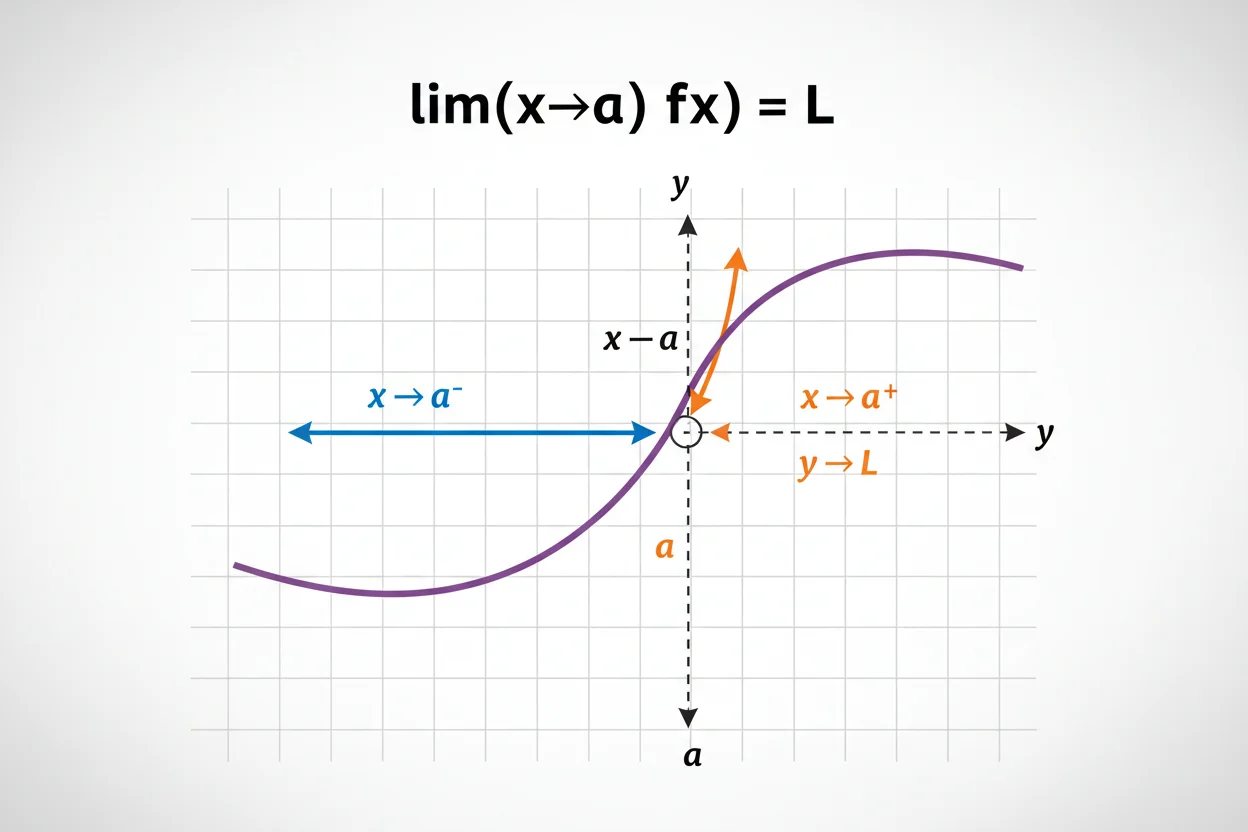
A limit describes the value a function approaches as its input approaches a particular point. The notation limₓ→ₐ f(x) = L means that f(x) can be made arbitrarily close to L by taking x sufficiently close to a, whether or not f(a) actually equals L. Limits allow calculus to describe behavior near a point rather than only at the point itself. They are the foundation of continuity, derivatives, definite integration, infinite processes, and many approximation methods. A limit may be evaluated by direct substitution when the function behaves regularly, but indeterminate forms such as 0/0 often require algebraic simplification before the approaching value becomes visible. Left-hand and right-hand behavior must agree for an ordinary two-sided limit to exist. A limit can also be infinite, or it can describe what happens as x itself grows without bound. The central question is always the same: what value does the function approach under the specified input behavior?
What Is a Limit?
Suppose:
limₓ→ₐ f(x) = L
This statement means:
as x approaches a, f(x) approaches L
The value of x does not have to equal a.
In fact, the function may even be undefined at x = a and still have a perfectly valid limit there.
For example:
f(x) = (x² − 4)/(x − 2)
is undefined at:
x = 2
because the denominator becomes zero.
However, for x ≠ 2:
(x² − 4)/(x − 2) = [(x − 2)(x + 2)]/(x − 2)
= x + 2
Therefore:
limₓ→₂ (x² − 4)/(x − 2) = 4
The missing function value does not prevent the nearby values from approaching 4.
Limit Notation
The expression:
limₓ→ₐ f(x) = L
contains three main pieces.
The input approaches:
a
The function being examined is:
f(x)
The output approaches:
L
For example:
limₓ→₃ (2x + 1) = 7
means that when x gets close to 3, the expression 2x + 1 gets close to 7.
Because this function is continuous at x = 3, direct substitution gives the answer immediately:
2(3) + 1 = 7
Direct Substitution
The first method to try when evaluating a limit is usually direct substitution.
Consider:
limₓ→₂ (x² + 3x − 1)
Substitute:
x = 2
Then:
2² + 3(2) − 1
= 4 + 6 − 1
= 9
Therefore:
limₓ→₂ (x² + 3x − 1) = 9
Polynomials are continuous everywhere, so their finite limits can be evaluated directly.
Limit of a Rational Function
Consider:
limₓ→₁ (x² + 2)/(x + 3)
Substitute:
x = 1
The numerator becomes:
1² + 2 = 3
The denominator becomes:
1 + 3 = 4
Therefore:
limₓ→₁ (x² + 2)/(x + 3) = 3/4
Direct substitution works because the denominator does not approach zero.
For rational functions, substitution is valid at points where the denominator remains nonzero.
When Direct Substitution Gives 0/0
Consider:
limₓ→₃ (x² − 9)/(x − 3)
Direct substitution produces:
0/0
This does not mean the limit is zero, undefined, or nonexistent.
The expression:
0/0
is an indeterminate form.
It tells us that the original expression must be simplified or analyzed further.
Factor the numerator:
x² − 9 = (x − 3)(x + 3)
So for x ≠ 3:
(x² − 9)/(x − 3) = x + 3
Now take the limit:
limₓ→₃ (x + 3) = 6
Therefore:
limₓ→₃ (x² − 9)/(x − 3) = 6
Factoring to Evaluate a Limit
Factoring is particularly useful when numerator and denominator share a factor that becomes zero at the limiting point.
Evaluate:
limₓ→₅ (x² − 25)/(x − 5)
Factor:
x² − 25 = (x − 5)(x + 5)
Cancel for x ≠ 5:
(x² − 25)/(x − 5) = x + 5
Therefore:
limₓ→₅ (x² − 25)/(x − 5)
= limₓ→₅ (x + 5)
= 10
The cancellation does not redefine the original function at x = 5. It reveals that the two expressions agree everywhere sufficiently close to 5 except at the point itself, which is all the limit requires.
Rationalizing a Limit
Radicals can create indeterminate forms that are simplified by multiplying by a conjugate.
Evaluate:
limₓ→₀ [√(x + 4) − 2]/x
Direct substitution gives:
0/0
Multiply numerator and denominator by the conjugate:
√(x + 4) + 2
Then:
[√(x + 4) − 2]/x × [√(x + 4) + 2]/[√(x + 4) + 2]
The numerator becomes:
(x + 4) − 4 = x
So:
= x/[x(√(x + 4) + 2)]
For x ≠ 0:
= 1/[√(x + 4) + 2]
Now substitute x = 0:
1/(2 + 2)
= 1/4
Therefore:
limₓ→₀ [√(x + 4) − 2]/x = 1/4
One-Sided Limits
A two-sided limit examines what happens from both sides of a point.
The left-hand limit is written conceptually as:
lim as x → a from the left of f(x)
The right-hand limit is:
lim as x → a from the right of f(x)
A two-sided limit:
limₓ→ₐ f(x)
exists only when both one-sided limits exist and are equal.
That condition is central to the wider theory of limits.
Example of Matching One-Sided Limits
Let:
f(x) = x + 2
As x approaches 1 from the left:
f(x) → 3
As x approaches 1 from the right:
f(x) → 3
Because both sides agree:
limₓ→₁ f(x) = 3
For ordinary continuous functions, this agreement happens automatically.
Example Where the Limit Does Not Exist
Define:
f(x) = −1 for x < 0
f(x) = 1 for x ≥ 0
As x approaches 0 from the left:
f(x) → −1
From the right:
f(x) → 1
Because:
−1 ≠ 1
the two-sided limit:
limₓ→₀ f(x)
does not exist.
This is a jump discontinuity.
The function’s assigned value at x = 0 does not repair the disagreement between the two sides.
Limit Versus Function Value
The statements:
limₓ→ₐ f(x) = L
and:
f(a) = L
are different statements.
A limit describes nearby behavior.
A function value describes what happens exactly at the point.
For example, define:
f(x) = x + 2 for x ≠ 1
and:
f(1) = 10
Then:
limₓ→₁ f(x) = 3
but:
f(1) = 10
The limit exists even though it does not equal the actual function value.
This distinction becomes essential when studying continuity.
Limit and Continuity
A function f is continuous at x = a when three conditions hold:
f(a) is defined
limₓ→ₐ f(x) exists
limₓ→ₐ f(x) = f(a)
So a limit is one component of continuity, but a limit by itself does not require the function to be defined at the target point.
For example:
(x² − 4)/(x − 2)
has limit 4 as x → 2 even though the original expression is undefined at x = 2.
Assigning:
f(2) = 4
would remove that removable discontinuity.
Basic Limit Laws
When the relevant limits exist, limits obey useful algebraic rules.
If:
limₓ→ₐ f(x) = L
and:
limₓ→ₐ g(x) = M
then the sum rule gives:
limₓ→ₐ [f(x) + g(x)] = L + M
The difference rule gives:
limₓ→ₐ [f(x) − g(x)] = L − M
For a constant c:
limₓ→ₐ [cf(x)] = cL
The product rule gives:
limₓ→ₐ [f(x)g(x)] = LM
The quotient rule gives:
limₓ→ₐ [f(x)/g(x)] = L/M
provided:
M ≠ 0
These rules allow complicated expressions to be broken into simpler pieces.
Power and Root Limit Rules
If:
limₓ→ₐ f(x) = L
then for a positive integer n:
limₓ→ₐ [f(x)]ⁿ = Lⁿ
Under the appropriate domain conditions, roots can also pass through the limit:
limₓ→ₐ √f(x) = √L
For example:
limₓ→₄ √(x + 5)
= √9
= 3
The continuity of the square-root function on its real domain justifies the substitution here.
Limit of a Polynomial
For any polynomial P:
limₓ→ₐ P(x) = P(a)
For example:
limₓ→₋₂ (3x³ − x + 5)
Substitute:
3(−8) − (−2) + 5
= −24 + 2 + 5
= −17
Therefore:
limₓ→₋₂ (3x³ − x + 5) = −17
Polynomial limits are among the simplest because no domain singularities occur.
Limit of a Quotient
If:
limₓ→ₐ f(x) = L
and:
limₓ→ₐ g(x) = M
with M ≠ 0, then:
limₓ→ₐ f(x)/g(x) = L/M
For example:
limₓ→₂ (x² + 1)/(3x − 1)
is:
(4 + 1)/(6 − 1)
= 5/5
= 1
The condition that the denominator’s limit is nonzero is essential.
The Squeeze Principle
Sometimes a function is difficult to evaluate directly but is trapped between two simpler functions approaching the same number.
If near a:
g(x) ≤ f(x) ≤ h(x)
and:
limₓ→ₐ g(x) = L
and:
limₓ→ₐ h(x) = L
then:
limₓ→ₐ f(x) = L
This is often called the squeeze theorem.
It is especially useful for oscillating expressions multiplied by something approaching zero.
Squeeze Example
Consider:
limₓ→₀ x² sin(1/x)
Because:
−1 ≤ sin(1/x) ≤ 1
multiplying by x² ≥ 0 gives:
−x² ≤ x² sin(1/x) ≤ x²
As x → 0:
−x² → 0
and:
x² → 0
Therefore:
limₓ→₀ x² sin(1/x) = 0
Even though sin(1/x) oscillates infinitely often near zero, the shrinking factor x² forces the product toward zero.
Infinite Limits
Sometimes a function grows without bound as x approaches a finite value.
For example:
f(x) = 1/x²
As x approaches 0 from either side:
1/x² → ∞
We write:
limₓ→₀ 1/x² = ∞
This notation does not mean infinity is a real number that the function reaches.
It means the function can be made arbitrarily large and positive by taking x sufficiently close to zero.
One-Sided Infinite Behavior
Consider:
f(x) = 1/x
As:
x → 0 from the right
we have:
1/x → ∞
But as:
x → 0 from the left
we have:
1/x → −∞
Because the two sides behave differently, there is no single two-sided finite or same-sign infinite limit at zero.
The line:
x = 0
is a vertical asymptote.
Limits at Infinity
A limit can also describe function behavior as x itself becomes arbitrarily large.
For example:
limₓ→∞ 1/x = 0
The function never needs to equal zero.
Instead, its values become as close to zero as desired for sufficiently large positive x.
Similarly:
limₓ→−∞ 1/x = 0
These are examples of limits at infinity.
Rational Function Limit at Infinity
Evaluate:
limₓ→∞ (3x² + 2x − 1)/(x² + 5)
Divide numerator and denominator by x²:
[3 + 2/x − 1/x²]/[1 + 5/x²]
As:
x → ∞
we have:
2/x → 0
1/x² → 0
5/x² → 0
Therefore:
limₓ→∞ (3x² + 2x − 1)/(x² + 5) = 3
For rational functions whose numerator and denominator have the same degree, the limit at ±∞ is the ratio of the leading coefficients.
Rational Functions With Different Degrees
For:
limₓ→∞ (2x + 1)/(x² + 4)
the denominator grows faster than the numerator.
Divide by x²:
[2/x + 1/x²]/[1 + 4/x²]
Every fraction in the numerator approaches zero, so:
limit = 0
By contrast:
(x³ + 1)/(x² + 1)
grows approximately like x, so its value does not approach a finite real number as x → ∞.
Comparing leading powers is often the fastest way to analyze rational limits at infinity.
Important Trigonometric Limit
One of the fundamental limits in calculus is:
limₓ→₀ sin x/x = 1
when x is measured in radians.
This result supports many trigonometric derivative formulas.
For example, it is used in deriving:
d/dx[sin x] = cos x
from the first-principles derivative definition.
The radian condition is essential; the corresponding numerical factor changes if angles are measured in another unit.
Related Trigonometric Limit
From:
limₓ→₀ sin x/x = 1
we also obtain:
limₓ→₀ x/sin x = 1
and, using standard identities:
limₓ→₀ (1 − cos x)/x = 0
These standard limits help simplify more complex trigonometric expressions near zero.
Limit and the Derivative
The derivative is defined using a limit.
For:
f′(x) = lim as h → 0 of [f(x + h) − f(x)]/h
the fraction is an average rate of change over a small interval.
The limit lets the interval width h approach zero, producing the instantaneous rate.
For example, with:
f(x) = x²
we obtain:
[f(x + h) − f(x)]/h
= [(x + h)² − x²]/h
Expand:
= [2xh + h²]/h
For h ≠ 0:
= 2x + h
Take the limit:
lim as h → 0 of (2x + h) = 2x
Therefore:
f′(x) = 2x
Without limits, the ordinary derivative cannot be defined in this way.
Limit and Linear Approximation
A linear approximation depends on the idea that a differentiable function becomes increasingly close to its tangent line at sufficiently small scales.
Near x = a:
f(x) ≈ f(a) + f′(a)(x − a)
The derivative itself comes from a limit, so the local accuracy of the tangent-line model is ultimately a limiting statement.
As:
x → a
the relative importance of higher-order deviations becomes smaller.
This is one reason limits are central to approximation theory.
Limit and Integration
The broader family of integrals is also grounded in limits.
A definite integral can be defined as the limit of increasingly fine sums:
Σ f(xᵢ*)Δx
As the largest subinterval width approaches zero, the sums approach the integral under appropriate conditions.
Thus differentiation uses a limit of difference quotients, while integration uses a limit of sums.
The two processes are then connected by the fundamental theorem of calculus.
Limit and Integration by Substitution
Integration by substitution is primarily a change-of-variable technique, but limits matter when transformed endpoints are infinite or approach singular values.
For example, if:
u = x²
and:
x → ∞
then:
u → ∞
A transformed improper integral must carry the correct limiting behavior into the new variable.
For ordinary finite substitutions, this issue is usually hidden because the transformed endpoints are regular numerical values.
Limit and Integration by Parts
Integration by parts can also interact with limits when used inside an improper integral.
For example, evaluating:
∫₀∞ xe^(−x) dx
requires replacing ∞ by a finite endpoint b, applying integration by parts, and then evaluating the limit as b → ∞.
Terms such as:
be^(−b)
must themselves be analyzed through limits.
So integration by parts handles the antiderivative structure, while the limit determines the improper endpoint behavior.
Limit and Improper Integrals
An improper integral is defined through one or more limits.
For example:
∫₁∞ 1/x² dx
means:
lim as b → ∞ of ∫₁ᵇ 1/x² dx
The finite integral becomes:
1 − 1/b
and:
lim as b → ∞ of (1 − 1/b) = 1
Therefore the improper integral converges to 1.
If the required limit is not finite, the improper integral diverges.
Limit and a Line Integral
A line integral accumulates a quantity along a curve.
Like other integrals, its rigorous construction can be understood through limits of sums over increasingly fine partitions of the curve.
For practical calculations, parameterization usually converts the problem into an ordinary definite integral.
The limiting foundation remains important conceptually, but evaluating one finite line integral normally uses established integration formulas rather than rebuilding the limiting definition each time.
Limit and Continuity From the Left and Right
For continuity at an interior point a:
lim as x → a from the left of f(x)
and:
lim as x → a from the right of f(x)
must both equal:
f(a)
At a domain endpoint, one-sided continuity may be used instead.
For example, if a function is defined only for x ≥ 0, continuity at x = 0 can be examined using the right-hand limit because values to the left are outside the domain.
This highlights the importance of the domain when interpreting a limit.
Limit and Piecewise Functions
Piecewise functions often require separate left- and right-hand calculations.
Consider:
f(x) = x + 2 for x < 1
f(x) = 4 − x for x ≥ 1
From the left:
lim as x → 1 from the left of f(x) = 3
From the right:
lim as x → 1 from the right of f(x) = 3
Therefore:
limₓ→₁ f(x) = 3
Since:
f(1) = 4 − 1 = 3
the function is also continuous at x = 1.
Piecewise Example With No Limit
Now define:
f(x) = x + 1 for x < 2
f(x) = x + 4 for x ≥ 2
From the left:
f(x) → 3
From the right:
f(x) → 6
Therefore:
limₓ→₂ f(x)
does not exist.
Changing the value f(2) would not fix the problem because the disagreement comes from the behavior of entire neighboring branches.
Removable Discontinuity
A removable discontinuity occurs when a finite limit exists but the function value is missing or different.
For:
f(x) = (x² − 1)/(x − 1)
the simplified expression for x ≠ 1 is:
x + 1
Therefore:
limₓ→₁ f(x) = 2
The original expression is undefined at x = 1.
Defining:
f(1) = 2
makes the extended function continuous there.
This is why a hole in a graph can have a well-defined limit.
Oscillating Limits
Some functions fail to approach any single value because they oscillate indefinitely.
A classic example is:
sin(1/x)
as:
x → 0
The argument 1/x grows without bound in magnitude, causing the sine function to oscillate endlessly between −1 and 1.
Therefore:
limₓ→₀ sin(1/x)
does not exist.
This differs from x²sin(1/x), where the squeeze theorem forces the oscillation into an increasingly narrow range around zero.
Infinite Limit Versus Limit at Infinity
These two ideas should not be confused.
An infinite limit such as:
limₓ→₀ 1/x² = ∞
describes output growing without bound while the input approaches a finite point.
A limit at infinity such as:
limₓ→∞ 1/x = 0
describes output behavior while the input itself grows without bound.
One often relates to vertical asymptotes; the other often relates to horizontal or oblique long-run behavior.
Limit Within Calculus and Linear Algebra
The limit is fundamentally a calculus concept within the broader Calculus & Linear Algebra framework.
It supports the definition of derivatives, continuity tests, integral constructions, infinite processes, and local approximation.
Linear algebra topics such as matrix operations do not require limits for their elementary definitions, but limits can enter when matrices or vectors vary continuously or when iterative processes are studied.
The core intent remains local or asymptotic function behavior.
Common Mistakes With Limits
A common mistake is assuming that substituting a value and obtaining 0/0 means the limit is zero. The form 0/0 is indeterminate and requires further analysis.
Another error is confusing:
limₓ→ₐ f(x)
with:
f(a)
They may be equal, but they do not have to be.
Students also sometimes check only one side of a point. A two-sided limit requires agreement from both directions.
Infinity should not be treated as an ordinary number that can simply be substituted into algebraic formulas.
Canceling a factor is valid only where that factor is nonzero; in a limit problem this can still be useful because the limiting process concerns nearby points rather than necessarily the target point itself.
Finally, when evaluating limits at infinity, compare growth rates rather than focusing on lower-degree terms that become negligible.
Frequently Asked Questions
What is a limit in calculus?
A limit is the value a function approaches as its input approaches a specified point or grows without bound.
What does limₓ→ₐ f(x) = L mean?
It means f(x) approaches L as x gets arbitrarily close to a.
Does x have to equal a when finding a limit?
No. A limit describes nearby behavior. The function may even be undefined at x = a.
What is the first method to try for a finite limit?
Direct substitution is usually the first step. If it gives an ordinary finite value, that is often the limit for continuous expressions.
What does 0/0 mean in a limit?
It is an indeterminate form. It signals that simplification, factoring, rationalization, or another method is needed.
When does a two-sided limit exist?
It exists when the left-hand and right-hand limits both exist and are equal.
Can a limit exist if the function value is undefined?
Yes. For example:
limₓ→₂ (x² − 4)/(x − 2) = 4
even though the original expression is undefined at x = 2.
What is an infinite limit?
It describes a function growing without bound as x approaches a point, such as:
limₓ→₀ 1/x² = ∞
What is a limit at infinity?
It describes long-run function behavior as x → ∞ or x → −∞.
Why are limits important?
They provide the foundation for continuity, derivatives, integration, asymptotic behavior, and local approximation.
How are limits related to derivatives?
A derivative is defined as a limit of difference quotients.
How are limits related to integrals?
Definite integrals can be defined as limits of increasingly fine sums, and improper integrals are defined using limits at infinite or singular bounds.




