Calculus & Linear Algebra: Complete Guide, Formulas & Examples

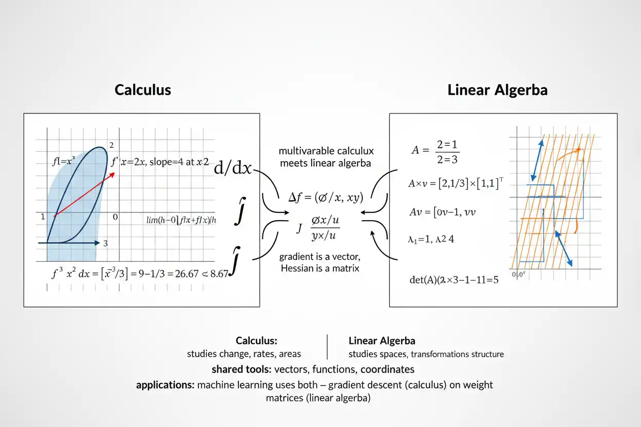
Calculus & linear algebra are two foundational branches of mathematics used to describe change, accumulation, multidimensional relationships, transformations, and systems of equations.

Calculus studies ideas such as:

limits,

derivatives,

integrals,

differential equations,

and:

multivariable change.

Linear algebra studies:

vectors,

matrices,

linear systems,

vector spaces,

transformations,

eigenvalues,

and:

eigenvectors.

The subjects become especially powerful when combined. Multivariable calculus uses vectors and matrices to describe derivatives in several dimensions, optimization uses gradients and curvature, differential equations often become matrix systems, and linear transformations provide the local structure behind many nonlinear problems.

This page provides the mathematical map. Narrow formulas and procedures belong to their specialist topics.

Calculus and Linear Algebra at a Glance

Calculus asks questions such as:

How fast is something changing?

What accumulated quantity results from a changing rate?

What happens as an input approaches a particular value?

Linear algebra asks:

How can several equations be solved together?

How do vectors combine?

How does a matrix transform space?

Which directions remain structurally important under a transformation?

Together, these subjects support mathematical models throughout science, engineering, economics, statistics, computing, optimization, and quantitative analysis.

Core Calculus Ideas

A useful conceptual progression is:

Limit → Derivative → Integral → Differential Equation

A limit describes local or asymptotic behavior.

A derivative measures instantaneous change.

An integral accumulates quantities.

A differential equation relates an unknown function to one or more of its derivatives.

Each stage builds on earlier ideas.

Limits

A limit describes the value a function approaches as its input approaches some point.

Typical notation is:

lim f(x) = L as x → a

The value L describes the behavior near a, whether or not the function itself equals L at that exact point.

For example:

f(x) = (x²−1)/(x−1)

For:

x ≠ 1

factor:

x²−1 = (x−1)(x+1)

so:

f(x) = x+1

Therefore as:

x → 1

the expression approaches:

2

The formula-first treatment belongs to Limit, while Limits covers the broader concept and interpretation.

Continuity

A function is continuous at a point when its value agrees with its limiting behavior there.

A standard condition at:

x = a

is:

lim f(x) = f(a) as x → a

Continuity connects local function behavior with derivative and integral theory.

The specialist continuity topic handles pointwise conditions, intervals, and discontinuities.

Derivatives

A derivative measures instantaneous rate of change.

One foundational definition is:

f′(x) = lim [f(x+h)−f(x)]/h as h → 0

Geometrically, f′(x) is the slope of the tangent line to the graph of f at that point.

For:

f(x) = x²

the derivative is:

f′(x) = 2x

So at:

x = 3

the instantaneous rate of change is:

6

The dedicated derivative page owns the main computational formula, while derivatives provides the wider conceptual treatment.

Power Rule

One of the most frequently used derivative rules is:

d/dx (xⁿ) = nx^(n−1)

For example:

d/dx (x⁵)

= 5x⁴

The power rule is the natural starting point for differentiating polynomial powers.

Product Rule

If:

y = f(x)g(x)

then:

y′ = f′g + fg′

For example:

y = x²eˣ

gives:

y′ = 2xeˣ + x²eˣ

The product rule applies when two differentiable functions are multiplied.

Quotient Rule

For:

y = f(x)/g(x)

with:

g(x) ≠ 0

the derivative is:

y′ = [f′g−fg′]/g²

The quotient rule organizes derivatives of ratios of functions.

Chain Rule

Composite functions require the chain rule:

d/dx f(g(x)) = f′(g(x))g′(x)

For example:

y = (3x+1)⁵

Then:

y′ = 5(3x+1)⁴ × 3

= 15(3x+1)⁴

The outer and inner changes both contribute.

Implicit Differentiation

Not every curve is initially written as:

y = f(x)

For:

x²+y² = 25

differentiate both sides with respect to x:

2x + 2y(dy/dx) = 0

Solve:

dy/dx = -x/y

This procedure is developed under implicit differentiation.

Differentials

A differential provides a linear description of a small change.

If:

y = f(x)

then:

dy = f′(x)dx

For small dx:

Δy ≈ dy

This idea connects derivative values with local change and is treated directly under differentials.

Linear Approximation

Near:

x = a

a differentiable function can be approximated by its tangent line:

f(x) ≈ f(a) + f′(a)(x−a)

For example, near:

x = 4

the function:

√x

has:

f(4)=2

and:

f′(4)=1/4

So near 4:

√x ≈ 2 + (x−4)/4

The linear approximation topic develops this local approximation technique.

Related Rates

When several quantities change together, derivatives can link their rates.

Suppose:

A = πr²

Differentiate with respect to time:

dA/dt = 2πr dr/dt

If:

r = 5

and:

dr/dt = 2

then:

dA/dt = 20π

The related rates framework focuses on identifying and connecting these time-dependent variables.

Optimization

Calculus often finds maximum and minimum values by locating critical points.

A common process is:

f′(x) = 0

then classify candidate points using sign behavior or higher derivatives.

For example:

f(x) = -x²+6x+2

Derivative:

f′(x) = -2x+6

Set:

-2x+6 = 0

giving:

x = 3

Because the quadratic opens downward, this point is a maximum.

The optimization topic owns these extremum methods and applied constraints.

Antiderivatives

An antiderivative reverses differentiation.

If:

F′(x) = f(x)

then:

F(x)

is an antiderivative of:

f(x)

For example:

f(x) = 2x

has antiderivatives:

F(x) = x² + C

where C is an arbitrary constant.

Indefinite Integrals

The notation:

∫ f(x) dx = F(x)+C

represents the family of antiderivatives.

For example:

∫ x² dx

= x³/3 + C

The indefinite integral focuses on this antiderivative interpretation, while the broader integrals topic connects indefinite and definite integration.

Definite Integrals

A definite integral accumulates a quantity across an interval:

∫ₐᵇ f(x) dx

When interpreted geometrically, it gives signed area between the graph and the horizontal axis.

If:

f(x) = x

from:

0 to 2

then:

∫₀² x dx

= [x²/2]₀²

= 2

The computational rules and interpretation belong to definite integral.

Fundamental Theorem of Calculus

The fundamental theorem of calculus connects differentiation and integration.

If:

F′(x)=f(x)

then:

∫ₐᵇ f(x) dx = F(b)−F(a)

This is one of the central structural results in calculus because it converts accumulation into antiderivative evaluation.

Area Under a Curve

For a nonnegative function over:

[a,b]

the area under a curve is:

A = ∫ₐᵇ f(x) dx

When a function crosses the axis, the integral gives signed area, so geometric area may require splitting the interval and handling signs appropriately.

Area Between Curves

If:

f(x) ≥ g(x)

on an interval:

[a,b]

then the area between curves is:

A = ∫ₐᵇ [f(x)−g(x)] dx

The essential setup is:

upper function − lower function

or, with horizontal slicing:

right function − left function.

Integration by Substitution

The integration counterpart of the chain rule is integration by substitution.

If:

u = g(x)

and:

du = g′(x)dx

then an integral can sometimes be rewritten in a simpler variable.

For example:

∫2x(x²+1)³ dx

let:

u = x²+1

so:

du = 2x dx

giving:

∫u³ du

= u⁴/4+C

= (x²+1)⁴/4+C

Integration by Parts

The integration by parts formula is:

∫u dv = uv − ∫v du

It is derived from the product rule and is useful when the integrand contains a product whose factors simplify under different operations.

Partial Fraction Integration

A rational function can sometimes be decomposed into simpler fractions before integration.

For example:

1/[(x−1)(x+1)]

can be split into terms involving:

1/(x−1)

and:

1/(x+1)

The systematic decomposition-and-integration process belongs to partial fraction integration.

Improper Integrals

An integral is improper when it involves an infinite interval or an unbounded integrand.

For example:

∫₁^∞ 1/x² dx

is interpreted as a limit.

It converges to:

1

The specialist improper integral topic determines when such limiting integrals converge or diverge.

Arc Length in Calculus

For a differentiable function:

y = f(x)

the arc length calculus formula over:

[a,b]

is:

L = ∫ₐᵇ √[1+(f′(x))²] dx

The derivative measures local slope, and the integral accumulates the resulting differential lengths.

Volumes of Revolution

Rotating a planar region around an axis creates three-dimensional solids.

Common methods include:

disks,

washers,

and:

cylindrical shells.

For example, the disk method often uses:

V = π∫ [R(x)]² dx

The specialist pages for volume by disks, volume by washers, and volume by shells own the setup rules for their respective geometries.

Surface Area of Revolution

A curve rotated around an axis can generate a surface rather than a solid volume.

A typical formula around the x-axis is:

S = 2π∫ y√[1+(dy/dx)²] dx

The geometry, bounds, and axis choice are handled under surface area of revolution.

Multivariable Calculus

Multivariable calculus extends calculus from functions of one variable to functions such as:

z = f(x,y)

or higher-dimensional mappings.

Instead of one ordinary derivative, several directional rates of change become possible.

This is where calculus begins to rely heavily on vectors and linear algebra.

Partial Derivatives

For:

f(x,y)

a partial derivative differentiates with respect to one variable while holding the others fixed.

For example:

f(x,y)=x²y+3y²

Then:

∂f/∂x = 2xy

and:

∂f/∂y = x²+6y

These separate rates combine into vector-valued derivative structures.

Gradient

The gradient collects first partial derivatives:

∇f = (∂f/∂x, ∂f/∂y, …)

For:

f(x,y)=x²+y²

we get:

∇f = (2x,2y)

The gradient points in the direction of steepest local increase and links multivariable calculus directly with vectors.

Directional Derivatives

If:

u

is a unit vector, the directional derivative of f in direction u is:

Dᵤf = ∇f · u

This formula explicitly combines a calculus object—the gradient—with a linear-algebra operation—the dot product.

Double Integrals

A double integral accumulates a function over a two-dimensional region:

∬ᴿ f(x,y) dA

Applications include:

area,

volume,

mass,

and:

probability.

The region R determines the integration bounds or geometry.

Triple Integrals

A triple integral extends accumulation to three dimensions:

∭ⱽ f(x,y,z) dV

These integrals can represent volume directly when:

f = 1

or accumulate density and other fields through a volume.

Line Integrals

A line integral accumulates a scalar or vector field along a curve.

A scalar-field form can be written:

∫ᶜ f ds

while vector-field work often involves:

∫ᶜ F · dr

The path itself becomes part of the integration problem.

Differential Equations

A differential equation contains an unknown function and one or more derivatives.

For example:

dy/dx = ky

has exponential solutions:

y = Ce^(kx)

Differential equations model quantities whose current rate of change depends on their current state or other variables.

Separable Differential Equations

A separable differential equation can be rearranged so the variables appear on opposite sides.

For:

dy/dx = g(x)h(y)

rewrite:

dy/h(y) = g(x)dx

Then integrate both sides.

This is one of the most accessible methods for solving first-order differential equations.

First-Order Linear Differential Equations

A first-order linear differential equation has standard form:

dy/dx + P(x)y = Q(x)

An integrating factor:

μ(x) = e^(∫P(x)dx)

can transform it into a form that integrates directly.

Euler Method

When an exact differential-equation solution is unavailable or unnecessary, Euler method constructs a numerical approximation.

For:

dy/dx = f(x,y)

with step size h:

yₙ₊₁ = yₙ + h f(xₙ,yₙ)

The method advances along local tangent-line estimates.

Core Linear Algebra Ideas

Linear algebra studies structures that preserve addition and scalar multiplication.

Its core objects include:

vectors,

matrices,

systems of linear equations,

vector spaces,

bases,

dimensions,

transformations,

eigenvalues,

and:

eigenvectors.

These objects encode multidimensional relationships in a form that is both algebraic and geometric.

Vectors

A vector can represent:

displacement,

direction,

force,

coordinates,

coefficients,

or a general element of a vector space.

A vector in three dimensions may be written:

v = (v₁,v₂,v₃)

The broader vector operations framework covers addition, subtraction, scalar multiplication, and related calculations.

Vector Magnitude

For:

v = (v₁,v₂,…,vₙ)

the Euclidean vector magnitude is:

||v|| = √(v₁²+v₂²+…+vₙ²)

For:

v = (3,4)

we get:

||v|| = √25

= 5

Magnitude connects linear algebra with geometry and square-root distance.

Dot Product

For vectors:

a = (a₁,…,aₙ)

and:

b = (b₁,…,bₙ)

the dot product is:

a·b = a₁b₁ + a₂b₂ + … + aₙbₙ

It also satisfies:

a·b = ||a||||b||cosθ

This connects vector coordinates with angles and orthogonality.

Vector Projection

The vector projection of a onto nonzero vector b is:

proj_b(a) = (a·b)/(b·b) b

Projection extracts the component of one vector lying in the direction of another.

It is fundamental to approximation, orthogonal decomposition, and least-squares reasoning.

Cross Product

For vectors in three-dimensional space, the cross product produces a vector perpendicular to both inputs.

If:

a × b = c

then:

c

is orthogonal to both:

a

and:

b

Its magnitude is:

||a×b|| = ||a||||b||sinθ

which also gives the area of the parallelogram generated by the two vectors.

Matrices

A matrix is a rectangular array of values.

For example:

A = [[1,2],[3,4]]

Matrices can represent:

systems of equations,

linear transformations,

data,

coefficients,

and:

multidimensional operators.

The broad matrix operations topic organizes the basic calculations.

Matrix Addition

Two matrices of the same dimensions are added entry by entry.

For:

A = [[1,2],[3,4]]

and:

B = [[5,6],[7,8]]

the matrix addition result is:

A+B = [[6,8],[10,12]]

Matrices with different dimensions cannot be added directly.

Matrix Multiplication

For:

A of size m×n

and:

B of size n×p

their matrix multiplication product:

AB

has size:

m×p

Each entry is a row-column dot product.

Matrix multiplication is generally:

not commutative

so:

AB

need not equal:

BA

even when both products exist.

Determinants

For a 2×2 matrix:

A = [[a,b],[c,d]]

the matrix determinant is:

det(A) = ad−bc

The determinant encodes scaling, orientation, and invertibility information.

For a square matrix:

det(A) ≠ 0

implies the matrix is invertible.

Matrix Inverse

For an invertible square matrix A, the matrix inverse satisfies:

AA⁻¹ = A⁻¹A = I

For:

A = [[a,b],[c,d]]

with:

ad−bc ≠ 0

the 2×2 inverse is:

A⁻¹ = 1/(ad−bc) [[d,−b],[−c,a]]

An inverse matrix reverses the associated linear transformation.

Row Reduction

A system of linear equations can be represented as an augmented matrix and simplified using elementary row operations.

The broader process of row reduction preserves the solution set while simplifying the matrix structure.

Typical row operations are:

swap two rows,

multiply a row by a nonzero scalar,

add a multiple of one row to another.

Reduced Row Echelon Form

Reduced row echelon form gives a canonical simplified matrix structure from which solution variables and dependencies can be identified directly.

A closely related formula-and-procedure treatment appears under RREF, where Gauss–Jordan elimination is the central computational process.

Matrix Rank

The matrix rank measures the number of linearly independent rows or columns.

Rank helps determine:

dimension of the image,

independence,

redundancy,

and:

whether systems have unique, infinite, or inconsistent solution structures.

For an m×n matrix:

rank(A) ≤ min(m,n)

Vector Spaces

A vector space is a collection of objects that can be added and multiplied by scalars while satisfying the standard vector-space axioms.

Vectors need not always be geometric arrows. They may be:

coordinate tuples,

polynomials,

matrices,

functions,

or other algebraic objects.

The structure matters more than the representation.

Basis and Dimension

A basis and dimension description identifies the independent directions required to represent a vector space.

A basis is a set of vectors that is:

linearly independent

and:

spanning.

The dimension is the number of vectors in any basis for a finite-dimensional space.

For ordinary three-dimensional space:

R³

a standard basis is:

(1,0,0)

(0,1,0)

(0,0,1)

and:

dimension = 3

Linear Transformations

A linear transformation preserves vector addition and scalar multiplication:

T(u+v)=T(u)+T(v)

T(cu)=cT(u)

With chosen bases, a finite-dimensional linear transformation can be represented by a matrix.

This is one of the central bridges between abstract vector spaces and concrete matrix computation.

Eigenvalues

For a square matrix:

A

an eigenvalue λ satisfies:

Av = λv

for some nonzero vector v.

The formula-first treatment is developed under eigenvalue, while eigenvalues covers the broader family of values and interpretation.

Eigenvalues are typically found from:

det(A−λI)=0

Eigenvectors

A nonzero vector v satisfying:

Av = λv

is an eigenvector corresponding to eigenvalue λ.

The focused calculation appears under eigenvector, while eigenvectors develops their collective interpretation and role in invariant directions.

Why Eigenvalues Matter

Under an ordinary matrix transformation, most vectors change both direction and magnitude.

An eigenvector instead remains on its own line:

Av = λv

Only its scale—and possibly direction sign—changes.

This makes eigenvectors and eigenvalues useful for:

repeated transformations,

dynamical systems,

differential equations,

stability,

principal directions,

and many other applications.

How Calculus and Linear Algebra Connect

The subjects become deeply intertwined in more than one dimension.

For a scalar function:

f:Rⁿ→R

the gradient is a vector.

For a vector-valued function:

F:Rⁿ→Rᵐ

its derivative is represented locally by a matrix of partial derivatives.

That matrix describes the best local linear approximation to the nonlinear function.

This is the central conceptual bridge:

Differentiation turns nonlinear behavior into a local linear transformation

Gradient as a Vector

For:

f(x,y)

the gradient is:

∇f = (fₓ,fᵧ)

This is a vector in the input space.

The direction:

∇f/||∇f||

when nonzero gives the direction of steepest increase.

The magnitude:

||∇f||

gives the maximum directional rate of change at that point.

Thus multivariable differentiation naturally produces linear-algebra objects.

Directional Derivative as a Dot Product

For unit vector u:

Dᵤf = ∇f·u

This formula combines:

partial derivatives from calculus

with:

the dot product from linear algebra.

If:

u

aligns with the gradient, the directional derivative is maximized.

If:

u

is perpendicular to the gradient, the directional derivative is zero.

Matrices as Derivatives

For a multivariable transformation:

F(x₁,…,xₙ)

the derivative at a point can be represented by a matrix containing partial derivatives.

This matrix maps small input changes to approximate output changes:

ΔF ≈ J Δx

where J is the derivative matrix.

This generalizes the one-variable linear approximation:

Δy ≈ f′(x)Δx

into several dimensions.

Linear Algebra in Differential Equations

A system:

x′ = Ax

uses both subjects directly.

The derivative:

x′

comes from calculus.

The matrix:

A

comes from linear algebra.

Eigenvalues and eigenvectors of A often determine characteristic growth, decay, oscillation, and stability directions.

This is one reason matrix theory becomes central in advanced differential-equation analysis.

Optimization in Several Variables

Suppose:

f(x,y)

must be optimized.

A candidate interior critical point often satisfies:

∇f = 0

That is:

∂f/∂x = 0

∂f/∂y = 0

Solving those equations may require algebraic or matrix techniques.

Higher-order behavior can then depend on a matrix of second derivatives.

Thus multivariable optimization is naturally both calculus and linear algebra.

Calculus vs. Linear Algebra

The two subjects emphasize different mathematical structures.

Calculus focuses primarily on:

change,

limits,

local approximation,

accumulation,

continuous models.

Linear algebra focuses primarily on:

linear combinations,

systems,

vector spaces,

transformations,

multidimensional structure.

But modern mathematical modeling often requires both.

A derivative is a local rate in one dimension and a local linear map in higher dimensions.

An integral can accumulate scalar or vector quantities.

A differential equation can evolve a vector state through a matrix.

A Basic Calculus Example

Let:

f(x)=x³−4x

Derivative:

f′(x)=3x²−4

At:

x=2

we get:

f′(2)=12−4

= 8

Therefore:

The instantaneous rate of change at x=2 is 8

The calculation is local: it describes how the function changes near one input.

A Basic Linear Algebra Example

Solve:

x+y=5

x−y=1

Add the equations:

2x=6

so:

x=3

Then:

y=2

In matrix form:

[[1,1],[1,−1]] [x,y]ᵀ = [5,1]ᵀ

Therefore:

(x,y)=(3,2)

Linear algebra organizes simultaneous relationships into vector and matrix form.

A Combined Example

Consider:

f(x,y)=x²+3y²

Gradient:

∇f=(2x,6y)

At:

(1,2)

we get:

∇f(1,2)=(2,12)

Now choose unit direction:

u=(0,1)

Directional derivative:

Dᵤf = (2,12)·(0,1)

= 12

Therefore:

The rate of change in the positive y-direction is 12

Calculus produced the gradient; linear algebra used the dot product to extract change in a chosen direction.

Common Mistake: Treating a Derivative as Only a Formula

A derivative is not merely a symbolic rule.

It represents:

local rate of change,

tangent slope,

and, in higher dimensions:

local linear approximation.

Understanding that meaning makes derivative formulas easier to apply correctly.

Common Mistake: Treating an Integral as Always Ordinary Area

A definite integral gives signed accumulation.

A region below the horizontal axis contributes negatively to:

∫f(x)dx

Geometric area may require absolute values or interval splitting.

Likewise, integrals can represent quantities other than area, including mass, work, probability, and volume.

Common Mistake: Assuming Matrix Multiplication Works Like Ordinary Multiplication

Matrix multiplication is dimension-dependent and generally noncommutative.

Even if both products exist:

AB ≠ BA

in general.

Order therefore matters.

Common Mistake: Assuming det(A)=0 Means Every Matrix Entry Is Zero

A zero determinant means a square matrix is singular.

It does not mean the matrix itself is the zero matrix.

For example:

[[1,2],[2,4]]

has determinant:

4−4=0

despite containing nonzero entries.

Common Mistake: Confusing Vectors With Magnitudes

A vector:

v=(3,4)

is not equal to its magnitude:

||v||=5

The vector includes direction and components.

The magnitude is a scalar.

Common Mistake: Using a Narrow Formula Outside Its Conditions

Mathematical formulas have assumptions.

For example:

matrix inverse requires invertibility,

logarithmic expressions require valid domains,

derivative rules require differentiability where applied,

geometric formulas require correct bounds,

improper integrals require limiting interpretation.

Checking conditions is part of the solution, not a separate optional step.

Frequently Asked Questions

What is calculus?

Calculus studies limits, rates of change, derivatives, integrals, and related continuous mathematical behavior.

What is linear algebra?

Linear algebra studies vectors, matrices, linear systems, vector spaces, transformations, eigenvalues, and related structures.

What is the derivative formula?

A foundational definition is:

f′(x)=lim [f(x+h)−f(x)]/h as h→0

What is a definite integral?

A definite integral:

∫ₐᵇ f(x)dx

represents signed accumulation over an interval.

How are derivatives and integrals connected?

The fundamental theorem of calculus connects integration with antiderivatives.

What is a vector?

A vector is an object that can be added to other vectors and multiplied by scalars; in coordinate space it is often represented by an ordered list of components.

What is a matrix?

A matrix is a rectangular array commonly used to represent systems and linear transformations.

What is matrix rank?

Rank is the number of linearly independent rows or columns of a matrix.

What is an eigenvalue?

An eigenvalue λ satisfies:

Av=λv

for some nonzero vector v.

What is an eigenvector?

It is a nonzero vector whose direction is preserved by a linear transformation, up to multiplication by its eigenvalue.

Where do calculus and linear algebra meet?

They meet prominently in multivariable calculus, optimization, differential equations, Jacobian matrices, gradients, directional derivatives, and local linear approximation.

Is calculus needed for linear algebra?

Elementary linear algebra can be studied independently of calculus. More advanced mathematical applications frequently use both.

Is linear algebra needed for multivariable calculus?

Basic multivariable calculations can begin without extensive linear algebra, but vectors, dot products, matrices, and transformations become increasingly important.

Final Perspective

Calculus and linear algebra answer complementary questions.

Calculus asks:

How does a quantity change or accumulate?

Linear algebra asks:

How do multidimensional quantities combine and transform?

Their central structures can be summarized as:

Derivative → instantaneous change

Integral → accumulation

Differential equation → evolution governed by rates

Vector → multidimensional quantity

Matrix → linear transformation or system representation

Eigenvalue/eigenvector → invariant scaling direction

In one variable, a derivative can look like a number.

In several variables, the derivative naturally becomes a linear object acting on changes in multiple directions.

That connection is why calculus and linear algebra appear together throughout advanced mathematics: calculus describes local and accumulated behavior, while linear algebra provides the language for organizing that behavior across dimensions.