


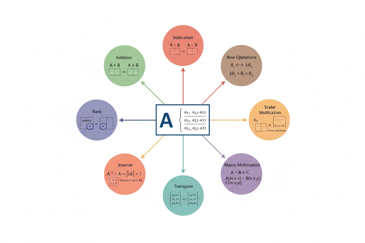
Matrix operations are the algebraic procedures used to combine, transform, and analyze matrices. Common operations include matrix addition and subtraction, scalar multiplication, matrix multiplication, transposition, row operations, determinants, inverses, powers, and rank calculations. Each operation has its own compatibility rules: addition requires matrices of identical dimensions, while multiplication requires the number of columns in the first matrix to equal the number of rows in the second. Some operations apply to rectangular matrices, while others such as ordinary determinants and inverses require square matrices. Matrix operations are closely connected because properties of one operation can determine whether another is possible—for example, a square matrix has an inverse exactly when its determinant is nonzero and its rank is full. Matrices can represent linear transformations, systems of equations, changes of coordinates, and multivariable derivative mappings, making these operations central to both linear algebra and applied mathematics. The first step in any matrix calculation is therefore to identify the requested operation and verify its dimensional requirements.
What Are Matrix Operations?
A matrix is a rectangular array of entries arranged into rows and columns.
For example:
A = [ 1 2 3 ]
[ 4 5 6 ]
has:
2 rows
and:
3 columns
so its dimensions are:
2×3
Matrix operations define what can be done with A by itself or in combination with other matrices.
The main elementary operations are:
- addition and subtraction,
- scalar multiplication,
- matrix multiplication,
- transpose,
- row operations,
- determinant calculation,
- matrix inversion,
- matrix powers,
- and rank determination.
Each operation answers a different mathematical question and follows different rules.
Matrix Dimensions
Before performing any matrix operation, determine the matrix dimensions.
If A has m rows and n columns, write:
A is m×n
For:
A = [ 2 4 ]
[ 1 3 ]
[ 5 7 ]
the matrix has:
3 rows
and:
2 columns
so:
A is 3×2
Dimensions determine whether addition, multiplication, inversion, and several other operations are defined.
Matrix Addition
Two matrices can be added only when they have identical dimensions.
If:
A = [aᵢⱼ]
and:
B = [bᵢⱼ]
then:
A + B = [aᵢⱼ + bᵢⱼ]
For example:
A = [ 1 2 ]
[ 3 4 ]
and:
B = [ 5 6 ]
[ 7 8 ]
give:
A + B = [ 6 8 ]
[ 10 12 ]
The dedicated matrix addition procedure handles the element-by-element calculation and its algebraic properties in detail.
Matrix Subtraction
Subtraction also requires equal dimensions.
It is defined as:
A − B = A + (−B)
Using:
A = [ 7 5 ]
[ 3 2 ]
and:
B = [ 2 1 ]
[ 4 −3 ]
we get:
A − B = [ 5 4 ]
[ −1 5 ]
Every entry in B is subtracted from the corresponding entry in A.
Unlike addition:
A − B ≠ B − A
in general.
Scalar Multiplication
A matrix can be multiplied by a scalar regardless of whether the matrix is square.
For scalar c:
cA = [caᵢⱼ]
Every entry is multiplied by the same scalar.
For example:
A = [ 1 −2 ]
[ 3 4 ]
Then:
3A = [ 3 −6 ]
[ 9 12 ]
Scalar multiplication preserves the dimensions of the matrix.
Negative of a Matrix
The additive inverse is obtained using scalar multiplication by −1:
−A = (−1)A
If:
A = [ 2 −5 ]
[ 1 3 ]
then:
−A = [ −2 5 ]
[ −1 −3 ]
This matrix satisfies:
A + (−A) = 0
where 0 is the same-sized zero matrix.
Matrix Multiplication
Standard matrix multiplication has a different compatibility rule.
If:
A is m×n
and:
B is n×p
then:
AB
is defined and has size:
m×p
Each entry is a row-column dot product:
cᵢⱼ = Σₖ₌₁ⁿ aᵢₖbₖⱼ
Matrix multiplication is therefore not performed by simply multiplying entries in identical positions.
Matrix Multiplication Example
Let:
A = [ 1 2 ]
[ 3 4 ]
and:
B = [ 2 0 ]
[ 1 5 ]
Then:
AB = [ 1(2)+2(1) 1(0)+2(5) ]
[ 3(2)+4(1) 3(0)+4(5) ]
So:
AB = [ 4 10 ]
[ 10 20 ]
This operation represents composition when matrices encode linear transformations.
Matrix Addition Versus Multiplication
The compatibility rules should not be confused.
For addition:
same dimensions required
Multiplication:
inner dimensions must match
For example:
2×3 + 2×3
is valid.
And:
(2×3)(3×4)
is valid.
But:
2×3 + 3×4
is not defined.
Likewise:
(2×3)(2×3)
is not defined under standard matrix multiplication.
Matrix Multiplication Is Not Usually Commutative
Matrix addition satisfies:
A + B = B + A
But matrix multiplication generally satisfies:
AB ≠ BA
In some cases one product may exist while the reversed product does not.
This means algebraic steps involving matrices must preserve multiplication order.
For example:
AX = B
cannot generally be rearranged as though A and X were ordinary numbers.
Associative Property
Matrix addition is associative:
(A + B) + C = A + (B + C)
Matrix multiplication is also associative when dimensions are compatible:
(AB)C = A(BC)
Therefore parentheses can change grouping without changing matrix order.
This property is especially useful when composing several transformations.
Distributive Properties
Matrix multiplication distributes over addition:
A(B + C) = AB + AC
and:
(A + B)C = AC + BC
Scalar multiplication also distributes:
c(A + B) = cA + cB
These rules make matrix expressions behave like ordinary algebra in some respects, even though multiplication remains noncommutative.
Transpose of a Matrix
The transpose of A, written:
Aᵀ
is obtained by turning rows into columns.
If:
A = [ 1 2 3 ]
[ 4 5 6 ]
then:
Aᵀ = [ 1 4 ]
[ 2 5 ]
[ 3 6 ]
A 2×3 matrix becomes a 3×2 matrix after transposition.
Transpose Rules
Important transpose identities include:
(Aᵀ)ᵀ = A
(A + B)ᵀ = Aᵀ + Bᵀ
(cA)ᵀ = cAᵀ
and:
(AB)ᵀ = BᵀAᵀ
Notice the reversed multiplication order in the final rule.
This reversal reflects how row and column roles switch under transposition.
Symmetric Matrices
A square matrix is symmetric when:
Aᵀ = A
For example:
A = [ 2 3 ]
[ 3 5 ]
is symmetric because the entries mirror across the main diagonal.
Real symmetric matrices have particularly useful eigenvalues and eigenvector properties, including real eigenvalues and orthogonal eigenvectors associated with distinct eigenvalues.
Identity Matrix
The identity matrix I is a square matrix with 1s along the main diagonal and 0s elsewhere.
For two dimensions:
I = [ 1 0 ]
[ 0 1 ]
It satisfies:
IA = A
and:
AI = A
when dimensions are compatible.
The identity is the multiplicative neutral element for square-matrix multiplication.
Zero Matrix
A zero matrix contains only zero entries.
For addition:
A + 0 = A
For compatible multiplication:
A0 = 0
and:
0A = 0
The dimensions of the zero matrix depend on the operation in which it appears.
Matrix Powers
For a square matrix A:
A² = AA
A³ = AAA
and:
Aⁿ
represents n repeated factors of A.
Also:
A⁰ = I
under the standard square-matrix convention.
Matrix powers are used to describe repeated state transitions, iterative models, and repeated linear transformations.
Matrix Determinant
The matrix determinant is a scalar associated with a square matrix.
For:
A = [ a b ]
[ c d ]
the determinant is:
det(A) = ad − bc
For example:
A = [ 3 1 ]
[ 2 4 ]
gives:
det(A) = 3(4) − 1(2)
= 10
A nonzero determinant means the square matrix is invertible.
What a Determinant Tells You
For a square matrix:
det(A) ≠ 0
means:
- the matrix has an inverse,
- the matrix has full rank,
- its columns are linearly independent,
- its rows are linearly independent,
- zero is not an eigenvalue.
By contrast:
det(A) = 0
means the matrix is singular.
Geometrically, its corresponding transformation collapses at least one dimension.
Matrix Inverse
A matrix inverse A⁻¹ satisfies:
AA⁻¹ = A⁻¹A = I
For:
A = [ a b ]
[ c d ]
with:
ad − bc ≠ 0
the 2×2 inverse is:
A⁻¹ = 1/(ad − bc) [ d −b ]
[ −c a ]
The inverse reverses the action of an invertible matrix.
Matrix Inverse Example
Let:
A = [ 2 1 ]
[ 1 1 ]
The determinant is:
2(1) − 1(1)
= 1
So:
A⁻¹ = [ 1 −1 ]
[ −1 2 ]
Verify:
AA⁻¹ = I
A zero determinant would make the inverse impossible.
Matrix Rank
The matrix rank is the number of linearly independent rows or columns of a matrix.
Equivalently, it is the dimension of the matrix’s column space.
For an m×n matrix:
rank(A) ≤ min(m, n)
For a square n×n matrix:
rank(A) = n
means full rank.
If:
rank(A) < n
the matrix is singular.
Rank Example
Consider:
A = [ 1 2 ]
[ 2 4 ]
The second row is:
2 × first row
so only one row direction is independent.
Therefore:
rank(A) = 1
The determinant is also:
1(4) − 2(2)
= 0
The determinant and rank conclusions agree.
Elementary Row Operations
Three elementary row operations are central to matrix calculations:
swap two rows
multiply a row by a nonzero scalar
add a multiple of one row to another
These operations can simplify matrices without changing the solution set of the corresponding linear system when performed correctly on an augmented matrix.
They form the basis of Gaussian elimination.
Row Swap
For:
[ 1 2 ]
[ 3 4 ]
swapping the rows gives:
[ 3 4 ]
[ 1 2 ]
A row swap changes the sign of a square matrix’s determinant.
It does not change the matrix rank.
Row Scaling
Multiplying one row by a nonzero number is another elementary operation.
For example:
R₂ → (1/2)R₂
changes:
[ 1 2 ]
[ 4 6 ]
to:
[ 1 2 ]
[ 2 3 ]
The rank remains unchanged.
For determinant calculations, scaling a row by k scales the determinant by k.
Row Replacement
The operation:
R₂ → R₂ − 3R₁
adds a multiple of one row to another.
This operation does not change the determinant.
It also preserves rank and the solution set of a linear system.
That makes row replacement especially convenient during elimination.
Row Echelon and Reduced Row Echelon Forms
Repeated row operations can convert a matrix into row echelon form or reduced row echelon form.
Reduced row echelon form makes pivots and free variables particularly clear.
It can be used to:
- solve systems,
- identify rank,
- find null-space relationships,
- and test invertibility.
The transformation is performed through row operations rather than ordinary entry-by-entry simplification.
Matrix Operations and Systems of Linear Equations
A linear system can be represented as:
Ax = b
where:
A = coefficient matrix
x = unknown vector
b = output vector
This matrix form connects several operations.
Matrix multiplication forms Ax.
Row operations solve the augmented system.
Rank determines consistency and independence.
An inverse can solve:
x = A⁻¹b
when A is invertible.
This is why matrix operations are often studied together rather than as isolated techniques.
Matrix Equation Example
Solve conceptually:
Ax = b
where:
A = [ 2 1 ]
[ 1 3 ]
and:
b = [5]
[7]
The determinant is:
2(3) − 1(1)
= 5
Since it is nonzero, A is invertible.
Therefore the system has one unique solution.
Using the inverse or row reduction gives:
x = 8/5
y = 9/5
The determinant tells us uniqueness before the actual solving step.
Matrix Operations and Linear Transformations
Matrices commonly represent linear transformations.
If:
T(x) = Ax
then multiplying by A applies the transformation.
Adding transformation matrices corresponds to adding compatible transformations.
Multiplying transformation matrices composes transformations.
An inverse matrix reverses an invertible transformation.
The determinant describes area or volume scaling for square transformations.
Rank describes the dimension of the resulting output space.
These interpretations give matrix operations geometric meaning.
Matrix Operations and Eigenvectors
An eigenvector satisfies:
Av = λv
The matrix operation being performed is multiplication, but the result has the special property that the output remains along the same vector direction.
The associated eigenvalue describes the scaling.
Eigenvectors therefore reveal particularly simple behavior hidden inside a matrix multiplication operation.
Matrix Operations and Eigenvalues
The eigenvalues of a square matrix are found through:
det(A − λI) = 0
This expression combines several matrix operations:
- scalar multiplication,
- matrix subtraction,
- determinant calculation.
Once an eigenvalue λ is known, its eigenvectors satisfy:
(A − λI)v = 0
The broader matrix framework therefore underlies the entire eigenvalue problem.
Matrix Operations and Basis
A basis provides coordinate directions for vectors and transformations.
If matrix A represents a transformation relative to one basis, a different basis can produce a different matrix representation of the same underlying map.
The concepts of basis and dimension explain why matrix columns, rank, and invertibility depend on linear independence.
Matrix operations then manipulate those coordinate representations.
Matrix Operations in Multivariable Calculus
Matrices also appear throughout multivariable calculus.
Partial derivatives of vector-valued functions can be organized into derivative matrices.
A local displacement can then be transformed through matrix multiplication to obtain a first-order output change.
Changes of coordinates, quadratic forms, systems of differential equations, and optimization methods can all involve matrix calculations.
This is one reason matrix fluency is valuable beyond standalone linear algebra.
Matrix Operations and Linear Approximation
For a vector-valued differentiable function, local behavior can often be approximated by:
Δy ≈ AΔx
where A is the derivative matrix.
This is a multivariable extension of linear approximation.
Matrix multiplication applies the local derivative mapping to the input displacement.
If the original mapping is itself linear, the formula becomes exact rather than approximate.
Matrix Operations and Optimization
Matrices arise naturally in optimization when several variables interact.
First derivatives can be organized through gradients, while second-order behavior can be represented by matrices of second derivatives.
Matrix rank, determinants, eigenvalues, and matrix multiplication can then help describe curvature and local behavior.
The underlying matrix operations remain the same even when the application is an optimization problem.
Matrix Operations and Differential Equations
Systems of differential equations can often be written:
x′ = Ax
Matrix multiplication describes the instantaneous system dynamics.
Eigenvalues and eigenvectors of A can reveal growth, decay, and invariant modes.
Matrix powers or exponential-related constructions can describe evolution through repeated or continuous transformations.
This shows how elementary matrix operations support more advanced mathematical models.
Matrix Operations and Matrix Shape
Different operations preserve or change matrix dimensions differently.
If A and B are m×n:
A + B is m×n
For scalar c:
cA is m×n
If:
A is m×n
then:
Aᵀ is n×m
If:
A is m×n
and:
B is n×p
then:
AB is m×p
Determinants and ordinary inverses require:
n×n
square matrices.
Keeping track of shape prevents many invalid operations.
Operation Compatibility Example
Suppose:
A is 2×3
B is 2×3
C is 3×4
Then:
A + B
is valid and gives:
2×3
The product:
AC
is valid:
(2×3)(3×4) → 2×4
But:
A + C
is not defined.
And:
CA
would require:
(3×4)(2×3)
whose inner dimensions 4 and 2 do not match.
Dimension analysis can resolve these questions before any arithmetic begins.
Matrix Operations and Determinant Rules
For square matrices:
det(AB) = det(A)det(B)
and:
det(A⁻¹) = 1/det(A)
when A is invertible.
But generally:
det(A + B) ≠ det(A) + det(B)
This demonstrates an important pattern: matrix operations interact through specific identities, not by blindly copying scalar arithmetic rules.
Matrix Operations and Inverse Rules
For invertible A and B:
(AB)⁻¹ = B⁻¹A⁻¹
But generally:
(A + B)⁻¹ ≠ A⁻¹ + B⁻¹
Similarly, if:
AX = B
then:
X = A⁻¹B
when A is invertible.
But for:
XA = B
the correct operation is:
X = BA⁻¹
The side on which a matrix multiplies matters.
Rank of Matrix Products
For compatible matrices:
rank(AB) ≤ min(rank(A), rank(B))
A product cannot create more independent dimensions than either factor provides.
If A is invertible square, then:
rank(AB) = rank(B)
and:
rank(BA) = rank(B)
because invertible multiplication changes coordinates without collapsing dimension.
This is one structural way rank interacts with multiplication.
Rank of Matrix Sums
For same-sized matrices:
rank(A + B) ≤ rank(A) + rank(B)
But equality is not guaranteed.
For example, if:
B = −A
then:
A + B = 0
which has rank zero.
Thus matrix addition can either increase, preserve, or reduce rank depending on the matrices involved.
Combining Matrix Operations
Consider:
C = 2A + 3B
If A and B have the same dimensions, first scale each matrix:
2A
and:
3B
then add their corresponding entries.
If the expression is:
C = A(B + D)
first verify that B and D can be added and that A can multiply their resulting matrix.
The order implied by parentheses matters.
Matrix expressions should be read structurally before arithmetic begins.
Example: Combined Addition and Multiplication
Let:
A = [ 1 0 ]
[ 2 1 ]
B = [ 2 1 ]
[ 0 3 ]
C = [ 1 1 ]
[ 1 0 ]
Find:
A(B + C)
First:
B + C = [ 3 2 ]
[ 1 3 ]
Now multiply:
A(B + C)
= [ 1 0 ] [ 3 2 ]
[ 2 1 ] [ 1 3 ]
The first row is:
(3, 2)
The second row is:
(2·3 + 1·1, 2·2 + 1·3)
= (7, 7)
Therefore:
A(B + C) = [ 3 2 ]
[ 7 7 ]
The distributive rule gives the same result through:
AB + AC
Order of Operations With Matrices
Parentheses should be respected first.
Scalar multiplication and matrix multiplication are then carried out before matrix addition or subtraction, subject to dimensional validity.
However, a matrix expression is not simply ordinary arithmetic with brackets.
Before calculating anything, verify that every operation exists.
For example:
A + BC
may be invalid even if BC itself is valid, because the dimensions of A may not match the dimensions of BC.
Checking Matrix Calculations
A good matrix calculation can often be checked structurally.
For addition, verify dimensions and corresponding positions.
For multiplication, verify:
inner dimensions match
and:
output has outer dimensions
For an inverse, check:
AA⁻¹ = I
And for a determinant, compare the result with invertibility or rank when those properties are known.
For row reduction, verify the row operations themselves rather than changing individual entries without a valid operation.
These checks often catch errors before complete recalculation is needed.
Common Matrix Operations Mistakes
A common mistake is assuming all matrices can be added or multiplied. Compatibility depends on dimensions.
Students may confuse elementwise multiplication with standard matrix multiplication.
Another frequent error is assuming:
AB = BA
Matrix multiplication is generally not commutative.
The determinant should not be calculated for an ordinary rectangular matrix.
A matrix with determinant zero does not have an ordinary inverse.
The additive inverse:
−A
must not be confused with the multiplicative inverse:
A⁻¹
Another common mistake is reversing neither order nor factors when taking the inverse or transpose of a product. The correct rules are:
(AB)⁻¹ = B⁻¹A⁻¹
(AB)ᵀ = BᵀAᵀ
Finally, matrix shape should be checked throughout multi-step calculations. Many otherwise plausible calculations are invalid because an intermediate operation has incompatible dimensions.
Frequently Asked Questions
What are matrix operations?
Matrix operations are procedures for combining, transforming, or analyzing matrices, including addition, subtraction, scalar multiplication, matrix multiplication, transpose, determinant, inverse, row operations, powers, and rank.
How do you add matrices?
Matrices must have the same dimensions. Add corresponding entries:
(A + B)ᵢⱼ = aᵢⱼ + bᵢⱼ
How do you subtract matrices?
Subtract corresponding entries:
A − B = A + (−B)
The matrices must have identical dimensions.
How do you multiply a matrix by a scalar?
Multiply every matrix entry by the scalar.
When can two matrices be multiplied?
For AB, the number of columns in A must equal the number of rows in B.
What dimensions does a matrix product have?
If:
A is m×n
and:
B is n×p
then:
AB is m×p
What is a matrix transpose?
The transpose Aᵀ is formed by turning the rows of A into columns.
What is a matrix determinant?
It is a scalar defined for square matrices that helps determine invertibility, rank, and geometric scaling.
When does a matrix have an inverse?
A square matrix has an ordinary inverse exactly when:
det(A) ≠ 0
equivalently, when it has full rank.
What is matrix rank?
Rank is the number of linearly independent row or column directions in a matrix.
What are elementary row operations?
They are row swaps, nonzero row scaling, and adding a multiple of one row to another.
Is matrix multiplication commutative?
Generally no:
AB ≠ BA
Is matrix addition commutative?
Yes, for same-sized matrices:
A + B = B + A
What is the difference between −A and A⁻¹?
−A is the additive inverse satisfying A + (−A) = 0. A⁻¹ is the multiplicative inverse satisfying AA⁻¹ = I.
How can I check which matrix operation to use?
Identify what the problem asks for, note every matrix dimension, verify the operation’s compatibility rule, and then apply the corresponding formula without borrowing rules from a different operation.




