


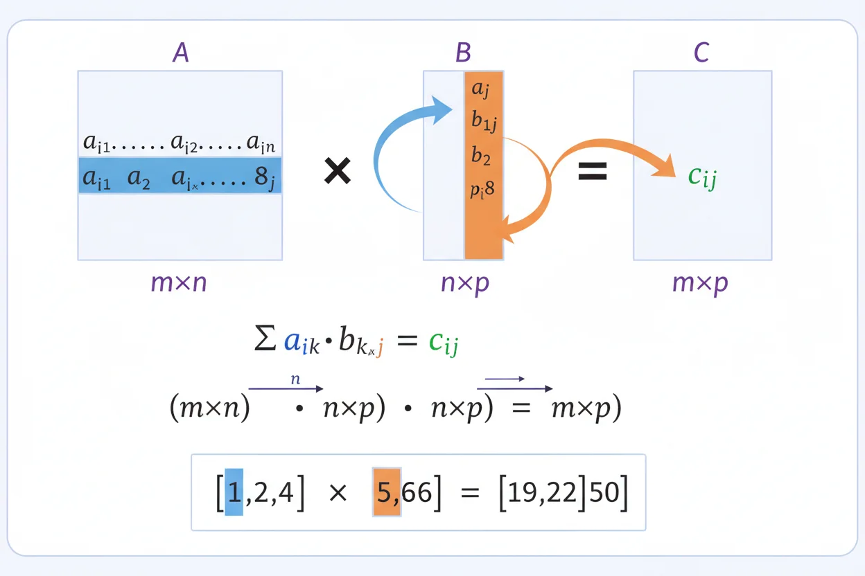
Matrix multiplication combines two matrices by taking dot products between rows of the first matrix and columns of the second. If A is an m×n matrix and B is an n×p matrix, then the product AB is defined and has dimensions m×p. The inner dimensions must match because every row of A must contain the same number of entries as every column of B. Each entry in the result is found by multiplying corresponding row and column entries and adding those products. Unlike matrix addition, matrix multiplication is not performed entry by entry, and order generally matters: AB usually does not equal BA. Matrix multiplication represents composition of linear transformations, powers repeated transformations, and provides the algebra behind systems, eigenvectors, inverses, and many computational models. Correctly identifying dimensions before multiplying is one of the simplest ways to prevent errors.
What Is Matrix Multiplication?
Suppose:
A = [aᵢⱼ]
and:
B = [bᵢⱼ]
To multiply A by B, the number of columns in A must equal the number of rows in B.
If:
A is m×n
and:
B is n×p
then:
AB is m×p
The entry in row i and column j of AB is obtained from row i of A and column j of B.
That entry is:
cᵢⱼ = aᵢ₁b₁ⱼ + aᵢ₂b₂ⱼ + … + aᵢₙbₙⱼ
or:
cᵢⱼ = Σₖ₌₁ⁿ aᵢₖbₖⱼ
The resulting matrix is:
C = AB
Matrix Multiplication Dimension Rule
The most important compatibility rule is:
(m×n)(n×p) → m×p
The two inner dimensions must match.
For example:
(2×3)(3×4) → 2×4
is valid.
But:
(2×3)(2×4)
is not defined because:
3 ≠ 2
A useful way to remember the rule is:
inner dimensions must agree; outer dimensions survive
So:
5×2 multiplied by 2×7
produces:
5×7
Basic 2×2 Matrix Multiplication
Let:
A = [ 1 2 ]
[ 3 4 ]
and:
B = [ 5 6 ]
[ 7 8 ]
To find AB, calculate each row-column dot product.
Top-left entry:
1(5) + 2(7)
= 5 + 14
= 19
Top-right entry:
1(6) + 2(8)
= 6 + 16
= 22
Bottom-left entry:
3(5) + 4(7)
= 15 + 28
= 43
Bottom-right entry:
3(6) + 4(8)
= 18 + 32
= 50
Therefore:
AB = [ 19 22 ]
[ 43 50 ]
Row-by-Column Rule
Every entry of a product matrix comes from one row of the left matrix and one column of the right matrix.
For:
C = AB
the entry:
c₂₃
comes from:
row 2 of A
and:
column 3 of B
If those vectors are:
(a₂₁, a₂₂, …, a₂ₙ)
and:
(b₁₃, b₂₃, …, bₙ₃)
then:
c₂₃ = a₂₁b₁₃ + a₂₂b₂₃ + … + a₂ₙbₙ₃
This is exactly a dot product between the selected row and column.
Example: 2×3 Times 3×2
Let:
A = [ 1 2 3 ]
[ 4 5 6 ]
and:
B = [ 7 8 ]
[ 9 10 ]
[ 11 12 ]
A is:
2×3
B is:
3×2
So:
AB
is defined and will be:
2×2
Calculate the top-left entry:
1(7) + 2(9) + 3(11)
= 7 + 18 + 33
= 58
Top-right:
1(8) + 2(10) + 3(12)
= 8 + 20 + 36
= 64
Bottom-left:
4(7) + 5(9) + 6(11)
= 28 + 45 + 66
= 139
Bottom-right:
4(8) + 5(10) + 6(12)
= 32 + 50 + 72
= 154
Therefore:
AB = [ 58 64 ]
[ 139 154 ]
Rectangular Matrix Example
Consider:
A = [ 2 1 ]
[ 0 3 ]
[ 4 −1 ]
which is:
3×2
and:
B = [ 5 2 1 ]
[ 1 0 −2 ]
which is:
2×3
Therefore:
AB
has dimensions:
3×3
First row:
2(5) + 1(1) = 11
2(2) + 1(0) = 4
2(1) + 1(−2) = 0
Second row:
0(5) + 3(1) = 3
0(2) + 3(0) = 0
0(1) + 3(−2) = −6
Third row:
4(5) + (−1)(1) = 19
4(2) + (−1)(0) = 8
4(1) + (−1)(−2) = 6
So:
AB = [ 11 4 0 ]
[ 3 0 −6 ]
[ 19 8 6 ]
Matrix Times a Column Vector
A matrix-vector product is an important special case of matrix multiplication.
Let:
A = [ 2 1 ]
[ 3 −2 ]
and:
v = [4]
[5]
Then:
Av = [ 2(4) + 1(5) ]
[ 3(4) − 2(5) ]
So:
Av = [13]
[2]
This is the standard coordinate form of a linear transformation.
Matrix Multiplication and Linear Transformations
Suppose:
T(x) = Ax
and:
S(x) = Bx
If T is applied first and S second:
S(T(x)) = B(Ax)
By associativity:
S(T(x)) = (BA)x
Therefore matrix multiplication represents composition of linear transformations.
The order is important.
The product:
BA
represents:
apply A first, then B
while:
AB
represents the reverse composition.
Matrix Multiplication Is Usually Not Commutative
For ordinary numbers:
ab = ba
But matrices generally satisfy:
AB ≠ BA
Consider:
A = [ 1 1 ]
[ 0 1 ]
and:
B = [ 1 0 ]
[ 1 1 ]
Calculate:
AB = [ 2 1 ]
[ 1 1 ]
Now reverse the order:
BA = [ 1 1 ]
[ 1 2 ]
Therefore:
AB ≠ BA
This noncommutativity is one of the most important distinctions between matrix and scalar multiplication.
Sometimes Only One Order Exists
Suppose:
A is 2×3
and:
B is 3×4
Then:
AB
is defined and has size:
2×4
But:
BA
would require multiplying:
(3×4)(2×3)
The inner dimensions are:
4 and 2
which do not match.
Therefore:
BA
is not even defined.
So reversing matrix order can change the result or make the product impossible.
Matrix Multiplication Is Associative
When dimensions are compatible:
(AB)C = A(BC)
This allows products of several matrices to be regrouped without changing their order.
For example:
ABC
can be calculated as either:
(AB)C
or:
A(BC)
The final matrix is identical.
However, choosing the more efficient grouping can reduce computational work when matrix dimensions vary greatly.
Matrix Multiplication Is Distributive
Matrix multiplication distributes over addition:
A(B + C) = AB + AC
and:
(A + B)C = AC + BC
when all dimensions are compatible.
For example, if B and C have the same dimensions and can both be multiplied on the left by A, then adding them before or after multiplication produces the same result.
This property connects matrix multiplication with the elementwise structure of matrix addition.
Scalar Multiplication and Matrix Products
For scalar k:
k(AB) = (kA)B = A(kB)
provided AB is defined.
For example, if:
A = [1 2]
and:
B = [3]
[4]
then:
AB = 11
Multiplying by 5:
5(AB) = 55
Alternatively:
(5A)B = [5 10][3, 4]ᵀ
= 15 + 40
= 55
The scalar can be attached to either matrix factor.
Identity Matrix and Multiplication
The identity matrix acts like the number 1.
For compatible square identity matrices:
IA = A
and:
AI = A
For:
A = [ a b ]
[ c d ]
the 2×2 identity matrix is:
I = [ 1 0 ]
[ 0 1 ]
Multiplying by I leaves every row and column combination unchanged.
This property is central to defining a matrix inverse.
Zero Matrix and Multiplication
If 0 is a compatible zero matrix:
A0 = 0
and:
0A = 0
However, an important difference from ordinary scalar algebra is that:
AB = 0
does not necessarily imply:
A = 0
or:
B = 0
Nonzero matrices can multiply to the zero matrix.
This is possible because singular matrices can collapse particular directions.
Example of Nonzero Matrices With Zero Product
Let:
A = [ 1 −1 ]
[ 1 −1 ]
and:
B = [ 1 1 ]
[ 1 1 ]
Both matrices are nonzero.
But:
AB = [ 0 0 ]
[ 0 0 ]
because every row-column product is:
1(1) + (−1)(1) = 0
This shows why cancellation rules require caution in matrix algebra.
Matrix Powers
For a square matrix A:
A² = AA
A³ = AAA
and generally:
Aⁿ = A·A·…·A
with n copies of A.
The zero power is defined as:
A⁰ = I
for the usual square-matrix convention.
Matrix powers describe repeated application of the same linear transformation.
Matrix Power Example
Let:
A = [ 2 0 ]
[ 0 3 ]
Then:
A² = [ 4 0 ]
[ 0 9 ]
and:
A³ = [ 8 0 ]
[ 0 27 ]
For a diagonal matrix, powers are especially simple because each diagonal value is raised independently.
Matrix Multiplication and Eigenvectors
If v is an eigenvector of A:
Av = λv
then repeated matrix multiplication gives:
A²v = λ²v
and generally:
Aⁿv = λⁿv
Thus matrix powers scale the eigenvector direction according to powers of the corresponding eigenvalue.
This is one reason eigenvalues are useful for understanding repeated transformations.
Eigenvalues of a Matrix Product
For square matrices A and B, the relationship between eigenvalues of AB and BA can be subtle.
When A and B are square of the same size, AB and BA have the same characteristic polynomial and therefore the same eigenvalues counting algebraic multiplicity.
However, arbitrary eigenvalues of A and B cannot generally be multiplied pairwise to obtain the eigenvalues of AB.
A simple product rule works only under additional structure, such as when a common eigenvector is involved.
Matrix Multiplication and Determinants
For square matrices:
det(AB) = det(A)det(B)
This property connects matrix multiplication with the matrix determinant.
If:
det(A) = 3
and:
det(B) = −2
then:
det(AB) = −6
Geometrically, the area- or volume-scaling factors of successive transformations multiply.
Product of Invertible Matrices
If A and B are invertible, then AB is invertible.
Its inverse is:
(AB)⁻¹ = B⁻¹A⁻¹
Notice the reversed order.
Check:
(AB)(B⁻¹A⁻¹)
= A(BB⁻¹)A⁻¹
= AIA⁻¹
= I
The inverse reverses the most recently applied transformation first.
Cancellation With Invertible Matrices
Suppose A is invertible and:
AB = AC
Multiply both sides on the left by A⁻¹:
A⁻¹AB = A⁻¹AC
So:
B = C
Thus left cancellation is valid when the cancelled matrix is invertible.
Without invertibility, cancellation may fail.
This illustrates why rank and determinant conditions matter even in seemingly simple matrix equations.
Matrix Multiplication and Rank
The matrix rank of a product satisfies:
rank(AB) ≤ min(rank(A), rank(B))
A product cannot have more independent output directions than either factor can support.
If one matrix is singular and collapses a dimension, later multiplication cannot generally recover the lost information.
For invertible square A:
rank(AB) = rank(B)
because multiplication by A changes coordinates without losing dimension.
Example of Rank Loss
Suppose:
A = [ 1 0 ]
[ 0 0 ]
This matrix projects vectors onto the x-axis.
Whatever compatible matrix B is multiplied on the right:
AB
cannot have rank greater than 1.
The first transformation A has already restricted every output to a one-dimensional subspace.
This geometric viewpoint makes the rank inequality intuitive.
Matrix Multiplication and Systems of Equations
A system of linear equations can be written:
Ax = b
The product Ax forms the linear combinations of the unknown entries specified by the rows of A.
For:
A = [ 2 1 ]
[ 3 −1 ]
and:
x = [x]
[y]
we obtain:
Ax = [ 2x + y ]
[ 3x − y ]
So the matrix equation:
Ax = [5]
[4]
is equivalent to:
2x + y = 5
3x − y = 4
Matrix multiplication therefore packages an entire linear system into one expression.
Matrix Multiplication and Basis
A matrix can represent how basis vectors are transformed.
If the columns of A are:
a₁, a₂, …, aₙ
then for:
x = (x₁, x₂, …, xₙ)
the matrix-vector product is:
Ax = x₁a₁ + x₂a₂ + … + xₙaₙ
This connects matrix multiplication directly with linear combinations and the concepts of basis and dimension.
The output is a weighted combination of the matrix columns.
Column Interpretation
Consider:
A = [ 1 4 ]
[ 2 5 ]
[ 3 6 ]
and:
x = [2]
[−1]
The columns are:
a₁ = (1, 2, 3)
a₂ = (4, 5, 6)
Therefore:
Ax = 2a₁ − a₂
= 2(1, 2, 3) − (4, 5, 6)
= (−2, −1, 0)
This is exactly what ordinary row-by-column multiplication produces.
Matrix Multiplication and Row Vectors
A row vector can multiply a compatible matrix from the left.
For:
u = [1 2]
and:
A = [ 3 4 5 ]
[ 6 7 8 ]
the product is:
uA
which has size:
(1×2)(2×3) → 1×3
Calculate:
uA = [1(3)+2(6), 1(4)+2(7), 1(5)+2(8)]
= [15, 18, 21]
Left and right multiplication therefore have different dimensional meanings.
Dot Products as Matrix Products
A row vector times a column vector produces a 1×1 matrix:
[a₁ a₂ … aₙ]
[b₁]
[b₂]
[…]
[bₙ]
The result is:
a₁b₁ + a₂b₂ + … + aₙbₙ
which is the dot product.
Thus matrix multiplication generalizes the dot-product operation across many rows and columns simultaneously.
Outer Products
A column vector times a row vector produces a matrix instead of a scalar.
For:
u = [1]
[2]
and:
vᵀ = [3 4 5]
the product is:
u****vᵀ
= [ 3 4 5 ]
[ 6 8 10 ]
This is called an outer product.
Its rank is at most 1 when both vectors are nonzero.
Transpose of a Product
For matrices with compatible dimensions:
(AB)ᵀ = BᵀAᵀ
The order reverses.
This resembles the inverse-of-a-product rule:
(AB)⁻¹ = B⁻¹A⁻¹
when inverses exist.
Order reversal appears because rows and columns swap roles under transposition.
Multiplication With Diagonal Matrices
Multiplying by a diagonal matrix can have a simple interpretation.
If D is diagonal, then:
DA
scales the rows of A according to the diagonal entries of D.
Meanwhile:
AD
scales the columns of A.
For example:
D = [ 2 0 ]
[ 0 3 ]
Then left multiplication:
DA
multiplies row 1 of A by 2 and row 2 by 3.
This distinction provides another example of why multiplication order matters.
Multiplication by a Permutation Matrix
A permutation matrix rearranges rows or columns.
Left multiplication by a permutation matrix rearranges rows.
Right multiplication rearranges columns.
For example, the matrix:
P = [ 0 1 ]
[ 1 0 ]
swaps two coordinates.
For:
A = [ a b ]
[ c d ]
the product:
PA = [ c d ]
[ a b ]
swaps the rows.
Meanwhile:
AP = [ b a ]
[ d c ]
swaps the columns.
Matrix Multiplication and Matrix Operations
The broader matrix operations framework includes addition, subtraction, scalar multiplication, multiplication, transposition, determinant, inverse, and row operations.
Matrix multiplication is distinguished by its row-column interaction and dimension compatibility rule.
It is not an entrywise operation.
Correctly identifying whether a problem asks for AB, BA, A+B, or a scalar multiple prevents many basic matrix errors.
Matrix Multiplication Versus Matrix Addition
For matrix addition:
dimensions must be identical
and:
result dimensions remain unchanged
For matrix multiplication:
columns of the first matrix must equal rows of the second
and:
result dimensions come from the outer dimensions
Example:
2×3 + 2×3 → 2×3
but:
(2×3)(3×5) → 2×5
The operations have fundamentally different compatibility rules.
Matrix Multiplication in Multivariable Calculus
In multivariable calculus, matrices can represent local derivative mappings for vector-valued functions.
Multiplying a derivative matrix by a small displacement vector produces a first-order approximation to the resulting output change.
Composition of differentiable mappings also leads to products of derivative matrices, which is a multivariable expression of the chain rule.
This provides a major connection between matrix multiplication and calculus.
Matrix Multiplication and Linear Approximation
A linear approximation of a vector-valued multivariable function may have form:
Δy ≈ AΔx
where A is the local derivative matrix.
Matrix multiplication converts the input displacement into the predicted first-order output displacement.
For a genuinely linear transformation, this relationship is exact rather than approximate:
y = Ax
Thus the same matrix product can describe either exact linear behavior or the first-order model of nonlinear behavior.
Matrix Multiplication and Reduced Row Echelon Form
Reduced row echelon form is produced using elementary row operations.
Those operations can themselves be represented by multiplication with elementary matrices.
If E represents one row operation, then:
EA
is the matrix obtained by applying that row operation to A.
A sequence of row operations corresponds to:
Eₖ…E₂E₁A
This connects elimination algorithms directly with matrix multiplication.
Order of Multiple Matrix Products
For:
ABC
the matrices must retain their original order.
Associativity allows:
(AB)C = A(BC)
but does not permit:
ABC = BAC
or any other arbitrary rearrangement.
Before multiplying several matrices, verify that the chosen grouping is dimensionally valid.
If the entire product is defined, associativity guarantees that any valid grouping gives the same result.
Common Matrix Multiplication Mistakes
The most common mistake is multiplying corresponding entries instead of using row-column dot products.
Another error is checking the wrong dimensions. For:
AB
compare:
columns of A
with:
rows of B
Students often assume:
AB = BA
because ordinary scalar multiplication is commutative. Matrix multiplication generally is not.
Another frequent error is constructing the result with the wrong dimensions. For:
(m×n)(n×p)
the answer must be:
m×p
Order reversal also matters for inverses and transposes:
(AB)⁻¹ = B⁻¹A⁻¹
(AB)ᵀ = BᵀAᵀ
Finally, arithmetic errors inside dot products are easy to make. Calculating one output entry at a time and keeping row-column pairs visually aligned makes verification easier.
Frequently Asked Questions
What is matrix multiplication?
Matrix multiplication combines rows of the first matrix with columns of the second using dot products.
What is the dimension rule for matrix multiplication?
If:
A is m×n
and:
B is n×p
then:
AB is m×p
When can two matrices be multiplied?
The number of columns in the first matrix must equal the number of rows in the second.
How do you find one entry of AB?
For:
C = AB
the entry cᵢⱼ is:
cᵢⱼ = Σₖ₌₁ⁿ aᵢₖbₖⱼ
Is matrix multiplication element by element?
No. Standard matrix multiplication uses row-column dot products.
Is matrix multiplication commutative?
Generally no:
AB ≠ BA
Is matrix multiplication associative?
Yes, when dimensions are compatible:
(AB)C = A(BC)
Does matrix multiplication distribute over addition?
Yes:
A(B + C) = AB + AC
and:
(A + B)C = AC + BC
What does multiplying a matrix by a vector mean?
It forms a linear combination of the matrix columns and represents the action of the associated linear transformation on that vector.
What does matrix multiplication represent geometrically?
It can represent successive linear transformations such as scaling, rotation, reflection, projection, or shear.
What is the determinant of a matrix product?
For square matrices:
det(AB) = det(A)det(B)
What is the inverse of a product?
If A and B are invertible:
(AB)⁻¹ = B⁻¹A⁻¹
How is matrix multiplication related to eigenvectors?
If Av = λv, then:
Aⁿv = λⁿv
so repeated matrix multiplication scales the eigenvector direction by successive powers of λ.
How can I check a matrix multiplication answer?
Verify the dimensions first, then recompute selected entries as row-column dot products. For special products, structural checks such as identity, determinant, or transformation behavior can provide additional confirmation.




