


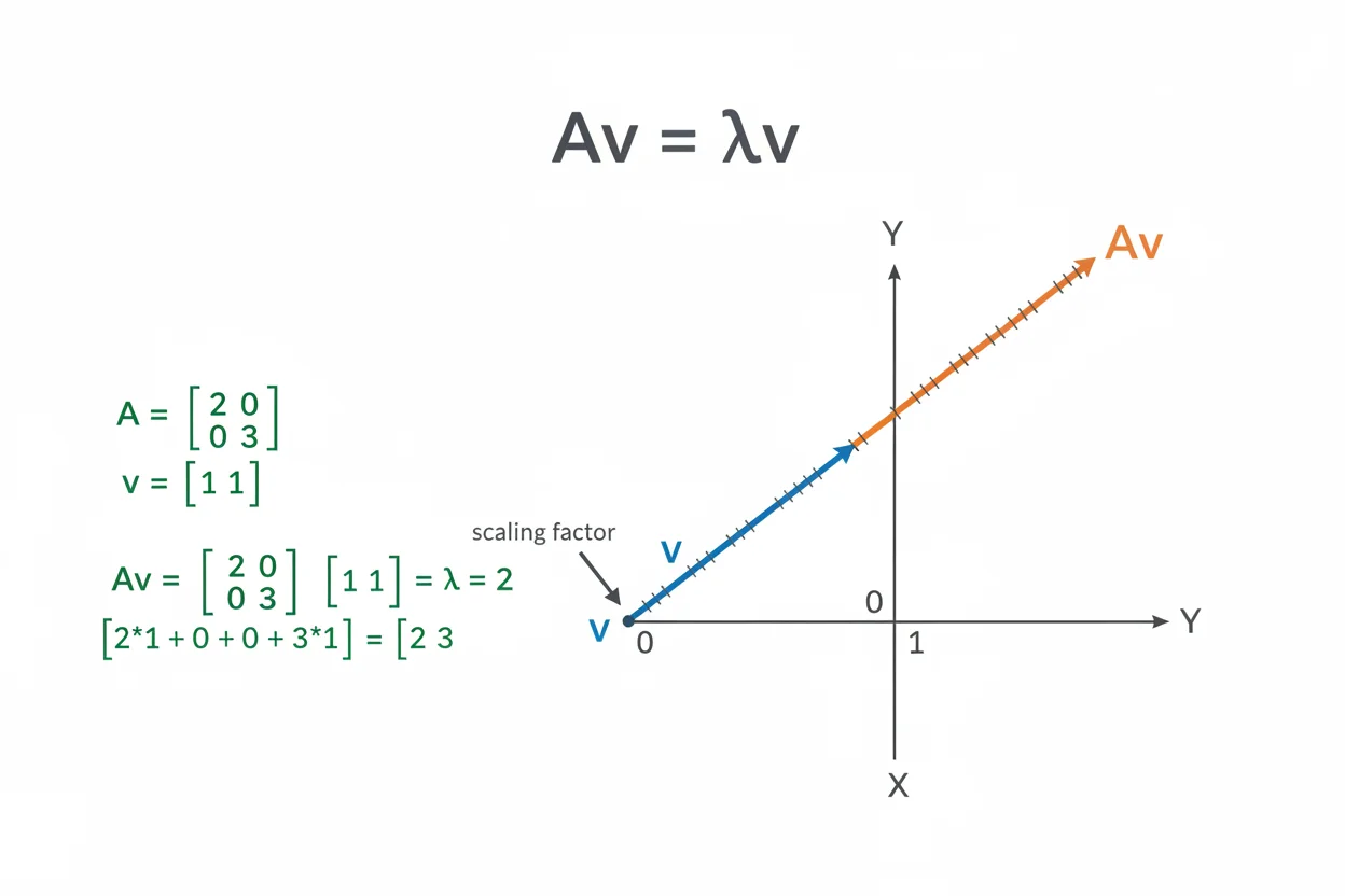
An eigenvector is a nonzero vector whose direction is preserved when a square matrix or linear transformation acts on it. If A is a matrix, v is an eigenvector when Av = λv for some scalar λ. The scalar λ is the corresponding eigenvalue and tells how much the eigenvector is stretched, shrunk, or reversed. To find an eigenvector, you normally determine an eigenvalue first and then solve (A − λI)v = 0 for a nonzero vector v. Any nonzero scalar multiple of an eigenvector is also an eigenvector associated with the same eigenvalue. Eigenvectors reveal the special directions in which a linear transformation acts by pure scaling rather than changing direction arbitrarily. They are useful for understanding matrix powers, systems of differential equations, repeated transformations, stability, and the structure of linear operators. For a 2×2 matrix, finding an eigenvector usually reduces to solving a small homogeneous system of linear equations.
What Is an Eigenvector?
Let A be a square matrix.
A nonzero vector v is an eigenvector of A if:
Av = λv
for some scalar λ.
The number λ is the corresponding eigenvalue.
The equation means that multiplying v by A gives a vector lying on the same line as v.
For example, suppose:
Av = 3v
Then v is an eigenvector and:
λ = 3
The transformation multiplies the length of v by 3 without reversing its direction.
If instead:
Av = −2v
then the eigenvector is scaled by 2 and reversed.
Eigenvector Formula
The defining formula is:
Av = λv
Move the right side to the left:
Av − λv = 0
Using the identity matrix I:
(A − λI)v = 0
This is the equation normally solved to find an eigenvector once λ is known.
Because v must not equal the zero vector, A − λI must be singular.
Therefore the associated eigenvalue satisfies:
det(A − λI) = 0
The determinant condition identifies λ, while the homogeneous system identifies v.
How to Find an Eigenvector
Suppose you are given a matrix A.
The standard process is:
- Find an eigenvalue λ from det(A − λI) = 0.
- Form A − λI.
- Solve (A − λI)v = 0.
- Choose any convenient nonzero solution.
- Verify Av = λv.
The first step belongs to the calculation of eigenvalues, while the remaining steps identify the associated direction.
Example: Find an Eigenvector
Consider:
A = [ 4 1 ]
[ 2 3 ]
Suppose we already know:
λ = 5
is an eigenvalue.
Form:
A − 5I
So:
A − 5I = [ −1 1 ]
[ 2 −2 ]
Let:
v = (x, y)
Then:
(A − 5I)v = 0
produces:
−x + y = 0
and:
2x − 2y = 0
Both equations are equivalent.
From:
−x + y = 0
we get:
y = x
Choose:
x = 1
Then:
y = 1
So one eigenvector is:
v = (1, 1)
Verify the Eigenvector
Multiply A by v:
Av = [ 4 1 ] [1]
[ 2 3 ] [1]
Using matrix multiplication:
Av = (4 + 1, 2 + 3)
= (5, 5)
Now calculate:
5v = 5(1, 1)
= (5, 5)
Therefore:
Av = 5v
The vector:
(1, 1)
is indeed an eigenvector corresponding to:
λ = 5
Finding Another Eigenvector of the Same Matrix
For:
A = [ 4 1 ]
[ 2 3 ]
the other eigenvalue is:
λ = 2
Form:
A − 2I = [ 2 1 ]
[ 2 1 ]
Solve:
2x + y = 0
Therefore:
y = −2x
Choose:
x = 1
Then:
y = −2
So an eigenvector is:
v = (1, −2)
Verify:
A(1, −2) = (4 − 2, 2 − 6)
= (2, −4)
and:
2(1, −2) = (2, −4)
Therefore:
Av = 2v
The vector is correct.
Why the Zero Vector Is Not an Eigenvector
The zero vector satisfies:
A0 = 0
for every matrix A.
It would also satisfy:
λ0 = 0
for every λ.
If the zero vector were allowed, every scalar would appear to work for every matrix, making the definition useless.
Therefore an eigenvector must satisfy:
v ≠ 0
This restriction is fundamental.
Scalar Multiples of an Eigenvector
If v is an eigenvector with eigenvalue λ, then every nonzero scalar multiple of v is also an eigenvector for the same eigenvalue.
Suppose:
Av = λv
Let c ≠ 0.
Then:
A(cv) = cAv
= cλv
= λ(cv)
Therefore:
cv
is also an eigenvector.
For example, if:
(1, 1)
is an eigenvector, then so are:
(2, 2)
(−3, −3)
(1/2, 1/2)
These vectors all represent the same eigendirection.
Eigenvector Direction Versus Length
An eigenvector is best understood as identifying a direction rather than one unique vector length.
If:
v
is an eigenvector, multiplying it by any nonzero scalar leaves it in the same eigenspace.
This is why answers to eigenvector problems may look different while still being equivalent.
For example:
(1, −2)
and:
(−3, 6)
describe the same eigenvector direction because:
(−3, 6) = −3(1, −2)
Both are valid.
Eigenvector and Eigenvalue Relationship
An eigenvector and its eigenvalue play different roles.
The eigenvector identifies a special direction.
The eigenvalue identifies how the transformation scales that direction.
The relationship is:
Av = λv
If:
λ > 1
the eigenvector grows in magnitude.
If:
0 < λ < 1
it shrinks.
If:
λ < 0
it reverses direction and is scaled by |λ|.
If:
λ = 0
the eigenvector is mapped to the zero vector.
Eigenvector for Eigenvalue Zero
Suppose:
λ = 0
Then:
Av = 0
So any corresponding eigenvector lies in the null space of A.
Because v is nonzero, this means A has a nontrivial null space.
The matrix is therefore singular.
Its matrix determinant is:
det(A) = 0
and it has no matrix inverse.
Thus a zero eigenvalue identifies directions that the transformation completely collapses.
Eigenvector and the Null Space
For a particular eigenvalue λ:
(A − λI)v = 0
The set of all solutions is the null space of:
A − λI
The nonzero vectors in that null space are eigenvectors corresponding to λ.
Therefore finding eigenvectors is fundamentally a homogeneous system of linear equations problem.
For a 2×2 matrix, this often reduces to one equation in two unknowns after the eigenvalue is substituted.
Example With a Free Variable
Let:
A = [ 3 2 ]
[ 0 3 ]
and consider:
λ = 3
Then:
A − 3I = [ 0 2 ]
[ 0 0 ]
Let:
v = (x, y)
The system gives:
2y = 0
so:
y = 0
The variable x is free.
Therefore:
v = (x, 0)
with:
x ≠ 0
Every nonzero vector on the x-axis is an eigenvector corresponding to λ = 3.
A convenient representative is:
v = (1, 0)
Eigenspace
The set consisting of the zero vector together with all eigenvectors associated with one eigenvalue is called an eigenspace.
For eigenvalue λ:
Eλ = null(A − λI)
Although the zero vector belongs to the eigenspace, it is not itself an eigenvector.
In the previous example:
E₃ = {(x, 0) : x is real}
This eigenspace is a one-dimensional subspace.
Its dimension is called the geometric multiplicity of λ.
Geometric Multiplicity
The geometric multiplicity of an eigenvalue is:
dimension of null(A − λI)
Equivalently, it is the number of linearly independent directions in that eigenvalue’s eigenspace.
For example, if:
A − λI
has a one-dimensional null space, the geometric multiplicity is 1.
If it has a two-dimensional null space, the geometric multiplicity is 2.
The geometric multiplicity cannot exceed the algebraic multiplicity of the corresponding eigenvalue.
Example of a Two-Dimensional Eigenspace
Consider:
A = [ 4 0 ]
[ 0 4 ]
For:
λ = 4
we have:
A − 4I = [ 0 0 ]
[ 0 0 ]
Every vector satisfies:
(A − 4I)v = 0
Therefore every nonzero vector in the plane is an eigenvector.
The eigenspace is two-dimensional.
This is a special case: the matrix is simply:
4I
and it scales every direction by 4.
Eigenvectors of Diagonal Matrices
Consider:
A = [ 2 0 ]
[ 0 5 ]
The standard basis vector:
e₁ = (1, 0)
satisfies:
Ae₁ = (2, 0)
= 2e₁
So e₁ is an eigenvector with:
λ = 2
Similarly:
e₂ = (0, 1)
satisfies:
Ae₂ = (0, 5)
= 5e₂
So e₂ corresponds to:
λ = 5
Diagonal matrices make eigenvector directions particularly easy to identify.
Eigenvectors of Triangular Matrices
For a triangular matrix, the eigenvalues can be read from the diagonal, but the eigenvectors still need to be found by solving:
(A − λI)v = 0
For example:
A = [ 2 1 ]
[ 0 4 ]
has eigenvalues:
2 and 4
For λ = 2:
A − 2I = [ 0 1 ]
[ 0 2 ]
which gives:
y = 0
so:
v = (1, 0)
is an eigenvector.
For λ = 4:
A − 4I = [ −2 1 ]
[ 0 0 ]
so:
y = 2x
and one eigenvector is:
(1, 2)
Eigenvectors and Linear Transformations
A matrix represents a linear transformation once a coordinate basis is chosen.
Most vectors can be turned into vectors pointing in new directions.
An eigenvector is special because:
Av = λv
keeps the result on the same line.
This makes eigenvectors a natural way to discover invariant directions within a transformation.
For a stretch along one axis, the axis direction may be an eigenvector. For a reflection, certain directions may have eigenvalues 1 or −1. For rotations through angles other than 0° or 180° in the real plane, real eigenvectors may not exist.
Eigenvectors and Basis
A collection of linearly independent eigenvectors can sometimes form a basis for the vector space.
The broader ideas of basis and dimension explain why this matters.
If an n×n matrix has n linearly independent eigenvectors, every vector can be expressed as a combination of those eigenvectors.
The transformation then acts particularly simply on those coordinates because each basis direction is scaled independently.
Distinct Eigenvalues and Independent Eigenvectors
Eigenvectors associated with distinct eigenvalues are linearly independent.
For the matrix:
A = [ 4 1 ]
[ 2 3 ]
we found:
λ₁ = 5 with v₁ = (1, 1)
and:
λ₂ = 2 with v₂ = (1, −2)
Because:
5 ≠ 2
the eigenvectors are linearly independent.
They can therefore form a basis for the two-dimensional space.
Repeated Eigenvalues
A repeated eigenvalue does not necessarily provide several independent eigenvectors.
Consider:
A = [ 3 1 ]
[ 0 3 ]
The only eigenvalue is:
λ = 3
with algebraic multiplicity 2.
But:
A − 3I = [ 0 1 ]
[ 0 0 ]
forces:
y = 0
so all eigenvectors are multiples of:
(1, 0)
There is only one independent eigenvector direction.
The plural eigenvectors topic considers the behavior of entire collections of eigenvectors and their independence more broadly.
Eigenvectors and Matrix Rank
The eigenvectors for λ satisfy:
(A − λI)v = 0
The matrix rank of A − λI determines the dimension of this null space.
For an n×n matrix:
nullity(A − λI) = n − rank(A − λI)
That nullity is the geometric multiplicity of λ.
Thus rank and eigenvector structure are directly connected.
Eigenvectors and Matrix Operations
Ordinary matrix operations do not generally preserve eigenvectors in simplistic ways.
If v is an eigenvector of A and B separately with:
Av = λv
and:
Bv = μv
then:
(A + B)v = (λ + μ)v
and:
ABv = λμv
But these formulas rely on v being a common eigenvector of both matrices.
Without that condition, eigenvectors of A + B or AB cannot usually be inferred by simply combining the eigenvectors of A and B.
Eigenvectors Under Matrix Powers
If:
Av = λv
then:
A²v = λ²v
and more generally:
Aⁿv = λⁿv
The eigenvector direction remains the same under every matrix power.
Only the scale factor changes.
This is one reason eigenvectors simplify repeated transformations.
For example, if:
λ = 0.5
then:
A¹⁰v = 0.5¹⁰v
so that component becomes very small after repeated applications.
Eigenvectors and the Dot Product
When matrices have orthogonal eigenvectors, their perpendicularity can be checked using the dot product.
If:
v₁ · v₂ = 0
the vectors are orthogonal.
Real symmetric matrices have particularly useful eigenvector structure: eigenvectors corresponding to distinct eigenvalues are orthogonal and can be normalized to produce an orthonormal basis.
This property is stronger than the general rule of mere linear independence.
Normalizing an Eigenvector
An eigenvector can be scaled to length 1.
If v is nonzero, its unit version is:
u = v/|v|
Suppose:
v = (3, 4)
Its vector magnitude is:
|v| = √(3² + 4²)
= 5
Therefore the normalized eigenvector is:
u = (3/5, 4/5)
Because u is a nonzero scalar multiple of v, it remains an eigenvector for the same eigenvalue.
Eigenvectors in Differential Equations
Systems of differential equations often have matrix form:
x′ = Ax
If:
Av = λv
then a solution associated with that eigenvector direction can take the form:
x(t) = e^(λt)v
Different eigenvectors can generate different modes of growth, decay, or oscillation.
This is one major application of eigenvectors outside purely algebraic matrix problems.
Eigenvectors and First-Order Numerical Methods
Eigenvectors are an exact linear-algebra concept, whereas the Euler method is a numerical procedure for approximating solutions of differential equations.
They can meet when a differential-equation system is represented by a matrix.
Eigenvectors may reveal the natural modes of the exact linear system, while Euler’s method approximates how the state evolves step by step.
These roles are complementary but distinct.
Eigenvectors Versus Double Integrals
A double integral accumulates values over a two-dimensional region:
∬ᴿ f(x, y) dA
An eigenvector is a direction preserved by a linear transformation.
Although both belong within the broader Calculus & Linear Algebra framework, they answer unrelated core questions: double integration concerns accumulation, while eigenvectors concern invariant directions under linear maps.
Example: Check Whether a Vector Is an Eigenvector
Let:
A = [ 5 2 ]
[ 0 3 ]
and consider:
v = (1, 0)
Calculate:
Av = (5, 0)
Since:
(5, 0) = 5(1, 0)
we have:
Av = 5v
Therefore:
v = (1, 0)
is an eigenvector with eigenvalue:
λ = 5
Now test:
w = (1, 1)
Then:
Aw = (7, 3)
For w to be an eigenvector, both components would need to equal the same scalar multiple of:
(1, 1)
But:
7 ≠ 3
No single λ satisfies:
(7, 3) = λ(1, 1)
Therefore w is not an eigenvector.
Example: Find an Eigenvector From a Known Eigenvalue
Let:
A = [ 6 2 ]
[ 2 3 ]
and suppose:
λ = 7
Form:
A − 7I = [ −1 2 ]
[ 2 −4 ]
Solve:
−x + 2y = 0
Therefore:
x = 2y
Choose:
y = 1
Then:
x = 2
So one eigenvector is:
v = (2, 1)
Verify:
A(2, 1) = (12 + 2, 4 + 3)
= (14, 7)
and:
7(2, 1) = (14, 7)
The result is correct.
Common Eigenvector Mistakes
A frequent error is allowing:
v = 0
as the solution. The zero vector must always be excluded when identifying eigenvectors.
Another mistake is solving:
Av = 0
for every eigenvalue. The correct system is:
(A − λI)v = 0
The eigenvalue must first be inserted.
Students sometimes think eigenvector answers must match one exact pair of numbers. Nonzero scalar multiples represent the same eigendirection and are all valid.
Another common error is finding λ correctly but failing to substitute it into the matrix before solving for v.
When verifying the result, every component of Av must equal the corresponding component of λv.
Finally, repeated eigenvalues should not be assumed to produce multiple independent eigenvectors automatically. The dimension of the eigenspace must be calculated.
Frequently Asked Questions
What is an eigenvector?
An eigenvector is a nonzero vector v satisfying:
Av = λv
for a square matrix A and scalar λ.
How do you find an eigenvector?
First find an eigenvalue λ. Then solve:
(A − λI)v = 0
and choose any nonzero solution.
Why can’t the zero vector be an eigenvector?
Because it satisfies A0 = λ0 for every λ, so allowing it would not identify any special direction or eigenvalue.
Can an eigenvector be multiplied by a constant?
Yes. Every nonzero scalar multiple of an eigenvector is another eigenvector for the same eigenvalue.
Are eigenvectors unique?
Usually not as individual vectors. Their direction is what matters, and every nonzero scalar multiple represents the same eigendirection.
What happens to an eigenvector under a matrix transformation?
It remains on the same line:
Av = λv
Its magnitude may increase, decrease, remain unchanged, or collapse to zero, and its direction may reverse if λ is negative.
What does eigenvalue zero mean for an eigenvector?
It means:
Av = 0
so the eigenvector belongs to the null space of A.
What is an eigenspace?
For eigenvalue λ, the eigenspace is:
null(A − λI)
It contains the zero vector and every eigenvector associated with λ.
Can one eigenvalue have many eigenvectors?
Yes. Every nonzero vector in its eigenspace is an eigenvector, so infinitely many scalar multiples usually exist.
Are eigenvectors for different eigenvalues independent?
Eigenvectors corresponding to distinct eigenvalues are linearly independent.
Can a repeated eigenvalue have only one eigenvector direction?
Yes. Its algebraic multiplicity can be greater than the dimension of its eigenspace.
How do I verify an eigenvector?
Calculate Av and λv. If the two vectors are identical and v is nonzero, the eigenvector is valid.




