


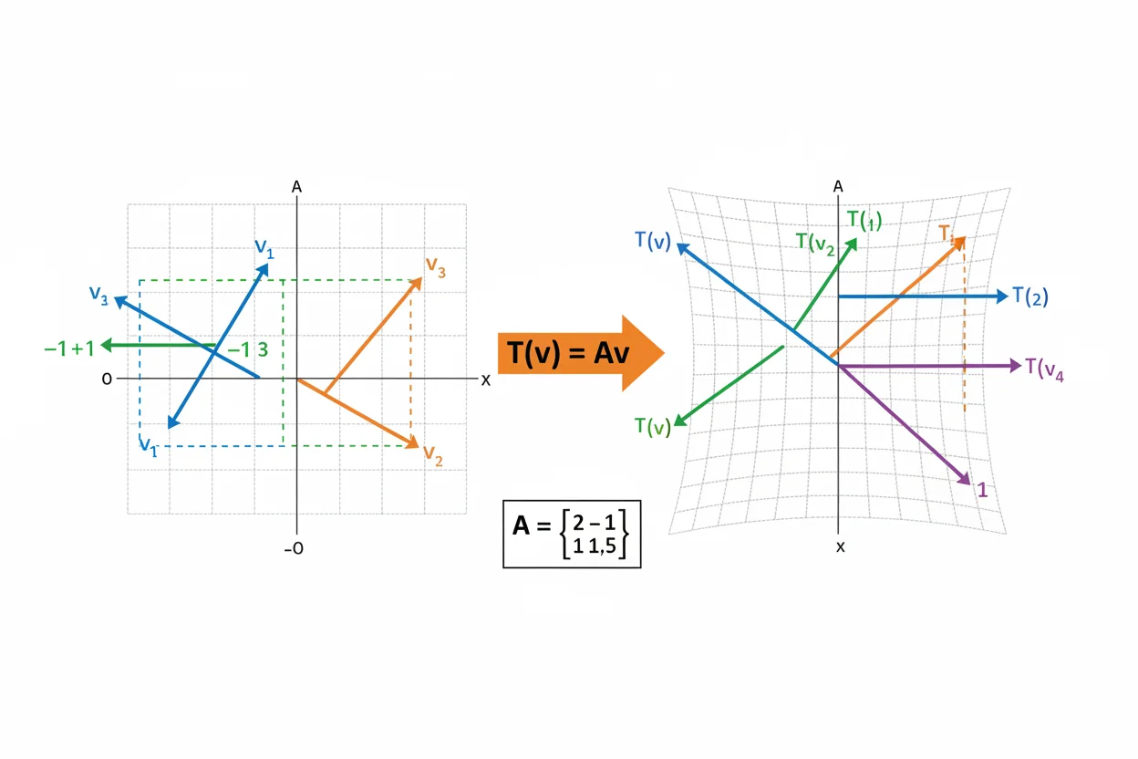
A linear transformation is a mapping between vector spaces that preserves vector addition and scalar multiplication. If T is linear, it must satisfy T(u + v) = T(u) + T(v) and T(cv) = cT(v) for every applicable pair of vectors and scalar c. In finite-dimensional coordinate spaces, a linear transformation can be represented by a matrix, so the transformation is often calculated as T(x) = Ax. Linear transformations can stretch, shrink, rotate, reflect, shear, project, or combine these effects while preserving the linear structure of the vector space. They always map the zero vector to the zero vector and preserve every linear combination of input vectors. A transformation can map between spaces of different dimensions, provided its matrix has the appropriate size. Properties such as kernel, range, rank, invertibility, determinant, and eigenstructure reveal how the transformation changes the space. Understanding linear transformations therefore connects vector geometry with matrix operations and provides one of the central organizing ideas of linear algebra.
What Is a Linear Transformation?
A transformation is a rule that maps vectors from one vector space to another.
Write:
T: V → W
where V is the domain and W is the codomain.
The transformation T is linear if it satisfies two rules.
For vectors u and v:
T(u + v) = T(u) + T(v)
For any scalar c:
T(cv) = cT(v)
These two conditions imply that T preserves every linear combination.
If:
x = c₁v₁ + c₂v₂ + … + cₙvₙ
then:
T(x) = c₁T(v₁) + c₂T(v₂) + … + cₙT(vₙ)
This preservation of linear combinations is the defining structure of a linear transformation.
Linear Transformation Formula
In coordinate form, a linear transformation is commonly represented as:
T(x) = Ax
where A is a matrix.
If:
A = [ a b ]
[ c d ]
and:
x = [ x ]
[ y ]
then:
T(x) = Ax
gives:
T(x, y) = (ax + by, cx + dy)
The calculation is ordinary matrix multiplication.
Each output coordinate is a linear combination of the input coordinates.
Example of a Linear Transformation
Let:
T(x, y) = (2x + y, x − 3y)
The corresponding matrix is:
A = [ 2 1 ]
[ 1 −3 ]
To transform:
v = (4, 2)
calculate:
T(4, 2) = (2·4 + 2, 4 − 3·2)
= (10, −2)
So:
T(4, 2) = (10, −2)
In matrix form:
[ 2 1 ] [4] = [10]
[ 1 −3 ] [2] [−2]
Testing the Addition Rule
For the same transformation:
T(x, y) = (2x + y, x − 3y)
let:
u = (1, 2)
and:
v = (3, −1)
First:
u + v = (4, 1)
Then:
T(u + v) = T(4, 1)
= (9, 1)
Now calculate the vectors separately:
T(1, 2) = (4, −5)
and:
T(3, −1) = (5, 6)
Add:
T(u) + T(v) = (4, −5) + (5, 6)
= (9, 1)
Therefore:
T(u + v) = T(u) + T(v)
The transformation satisfies the addition condition.
The underlying vector sum is closely related to matrix addition when transformations themselves are represented by matrices.
Testing the Scalar Rule
Use:
T(x, y) = (2x + y, x − 3y)
with:
v = (1, 2)
and:
c = 4
Calculate:
4v = (4, 8)
Then:
T(4, 8) = (16, −20)
Now find:
T(1, 2) = (4, −5)
and multiply by 4:
4T(1, 2) = 4(4, −5)
= (16, −20)
Therefore:
T(4v) = 4T(v)
The scalar-multiplication condition also holds.
One Combined Linearity Rule
The two defining rules can be combined into one statement.
For scalars a and b:
T(au + bv) = aT(u) + bT(v)
If this relationship holds for every relevant choice of vectors and scalars, T is linear.
This form often makes proofs and calculations more concise.
Every Linear Transformation Maps Zero to Zero
A linear transformation must satisfy:
T(0) = 0
To see why, write:
0 = 0v
Then:
T(0) = T(0v)
By scalar preservation:
T(0v) = 0T(v)
Therefore:
T(0) = 0
This provides a quick test for nonlinearity.
If a transformation maps the zero vector to anything other than zero, it cannot be linear.
Example of a Nonlinear Transformation
Consider:
T(x, y) = (2x + 1, y)
Evaluate the zero vector:
T(0, 0) = (1, 0)
Since:
T(0, 0) ≠ (0, 0)
the transformation is not linear.
The constant term +1 causes the failure.
A transformation containing a nonzero translation generally does not satisfy the strict linearity conditions.
Another Nonlinear Example
Consider:
T(x, y) = (x², y)
The first component contains x².
Check scalar multiplication:
T(2x, 2y) = (4x², 2y)
but:
2T(x, y) = (2x², 2y)
These are not generally equal.
Therefore the transformation is nonlinear.
The word “linear” requires more than simply having a visually simple formula.
Matrix Representation
Every linear transformation:
T: Rⁿ → Rᵐ
can be represented by an:
m × n
matrix A such that:
T(x) = Ax
The number of matrix columns equals the dimension of the input space.
The number of rows equals the dimension of the output space.
For example:
A = [ 1 2 3 ]
[ 4 5 6 ]
defines a transformation:
T: R³ → R²
because the matrix accepts three-component vectors and returns two-component vectors.
How to Find the Matrix of a Transformation
Suppose:
T: R² → R²
The standard basis vectors are:
e₁ = (1, 0)
e₂ = (0, 1)
The matrix of T is formed by placing their transformed vectors in columns:
A = [ T(e₁) T(e₂) ]
For example, suppose:
T(1, 0) = (2, 3)
and:
T(0, 1) = (−1, 4)
Then:
A = [ 2 −1 ]
[ 3 4 ]
Therefore:
T(x, y) = A[x, y]ᵀ
which gives:
T(x, y) = (2x − y, 3x + 4y)
Why Basis Vectors Determine the Transformation
Every vector in R² can be written:
(x, y) = xe₁ + ye₂
By linearity:
T(x, y) = xT(e₁) + yT(e₂)
Therefore, once the transformation of each basis vector is known, the transformation of every vector is determined.
This is one reason basis and dimension are fundamental to linear transformations.
The same principle extends to any finite-dimensional vector space.
Scaling Transformation
Consider:
T(x, y) = (2x, 3y)
Its matrix is:
A = [ 2 0 ]
[ 0 3 ]
The transformation stretches x-coordinates by a factor of 2 and y-coordinates by a factor of 3.
For:
(1, 2)
we get:
T(1, 2) = (2, 6)
This is a linear transformation because both coordinates are multiplied by constants and no translations or nonlinear terms are introduced.
Uniform Scaling
If:
T(v) = cv
for every vector v, then the matrix is:
cI
where I is the identity matrix.
For example:
T(x, y) = (4x, 4y)
has matrix:
[ 4 0 ]
[ 0 4 ]
Every direction is preserved, while every length is multiplied by 4.
Rotation Transformation
A counterclockwise rotation by angle θ in R² has matrix:
R = [ cos θ −sin θ ]
[ sin θ cos θ ]
Therefore:
T(x, y) = (x cos θ − y sin θ, x sin θ + y cos θ)
For:
θ = 90°
we have:
cos 90° = 0
sin 90° = 1
so:
R = [ 0 −1 ]
[ 1 0 ]
Thus:
T(x, y) = (−y, x)
For example:
T(3, 1) = (−1, 3)
The vector is rotated 90° counterclockwise.
Reflection Transformation
Reflection across the x-axis is:
T(x, y) = (x, −y)
Its matrix is:
A = [ 1 0 ]
[ 0 −1 ]
For:
(3, 4)
the result is:
(3, −4)
Reflection preserves linear combinations and is therefore linear.
Projection Transformation
Projection onto the x-axis is:
T(x, y) = (x, 0)
with matrix:
A = [ 1 0 ]
[ 0 0 ]
For:
(3, 5)
we obtain:
(3, 0)
This transformation removes the vertical component.
Projection is linear even though it loses information and is not invertible.
Shear Transformation
A horizontal shear can be written:
T(x, y) = (x + ky, y)
with matrix:
A = [ 1 k ]
[ 0 1 ]
If:
k = 2
then:
T(x, y) = (x + 2y, y)
For:
(1, 3)
we obtain:
(7, 3)
The y-coordinate remains unchanged while horizontal position depends on y.
Identity Transformation
The identity transformation leaves every vector unchanged:
T(v) = v
Its matrix is the identity matrix:
I
In R²:
I = [ 1 0 ]
[ 0 1 ]
Thus:
I(x, y) = (x, y)
The identity transformation plays the same neutral role in composition that the number 1 plays in multiplication.
Zero Transformation
The zero transformation maps every vector to zero:
T(v) = 0
In R² its matrix is:
[ 0 0 ]
[ 0 0 ]
This transformation is linear because:
T(u + v) = 0
and:
T(u) + T(v) = 0 + 0
= 0
It is an extreme example of a transformation that collapses all dimensions.
Kernel of a Linear Transformation
The kernel is the set of vectors mapped to zero:
ker(T) = {v : T(v) = 0}
If:
T(x) = Ax
then the kernel consists of solutions to:
Ax = 0
For example, consider:
T(x, y) = (x + y, 2x + 2y)
To belong to the kernel:
x + y = 0
So:
y = −x
Therefore:
ker(T) = {(x, −x)}
The kernel reveals which input directions are completely lost.
Range of a Linear Transformation
The range, or image, is the set of all possible outputs:
range(T) = {T(v) : v in the domain}
If T is represented by A, the range is the column space of A.
The dimension of this range is the matrix rank.
A transformation from Rⁿ to Rᵐ may fill the entire codomain or only a lower-dimensional subspace.
Rank and Nullity
For a linear transformation:
T: Rⁿ → Rᵐ
the rank-nullity relationship is:
rank(T) + nullity(T) = n
Here:
rank(T) = dimension of range(T)
and:
nullity(T) = dimension of ker(T)
This relationship shows how the input dimensions divide between directions preserved in the output and directions collapsed to zero.
Invertible Linear Transformation
A linear transformation:
T: Rⁿ → Rⁿ
is invertible when there is another transformation T⁻¹ satisfying:
T⁻¹(T(v)) = v
If:
T(v) = Av
then T is invertible exactly when A has a matrix inverse.
For a square matrix, this requires:
det(A) ≠ 0
and full rank.
An invertible transformation neither collapses distinct vectors together nor leaves any output direction unreachable.
Determinant and Geometric Scaling
For a square transformation matrix A, the matrix determinant provides geometric information.
In two dimensions:
|det(A)|
is the factor by which areas are scaled.
In three dimensions:
|det(A)|
is the factor by which volumes are scaled.
If:
det(A) = 0
the transformation collapses the space into a lower-dimensional set.
If the determinant is negative, orientation is reversed in addition to the magnitude scaling.
Example Using the Determinant
Consider:
A = [ 2 0 ]
[ 0 3 ]
Then:
det(A) = 2·3
= 6
So the transformation scales two-dimensional area by:
6
A unit square is transformed into a rectangle of area 6.
Because the determinant is nonzero, the transformation is invertible.
Eigenvectors of a Linear Transformation
An eigenvector is a nonzero vector whose direction is preserved under a linear transformation:
T(v) = λv
The scalar λ is the corresponding eigenvalue.
Eigenvectors identify special directions along which the transformation acts only by scaling or reversal.
For example, a projection onto the x-axis has:
(1, 0)
as an eigenvector with eigenvalue:
1
while:
(0, 1)
is an eigenvector with eigenvalue:
0
The first direction is preserved, while the second is collapsed.
Composition of Linear Transformations
Suppose:
T(x) = Ax
and:
S(x) = Bx
Applying T first and then S gives:
S(T(x)) = B(Ax)
Therefore:
S ∘ T
has matrix:
BA
Composition of linear transformations corresponds to matrix multiplication.
Order matters because:
BA
does not generally equal:
AB
Example of Composition
Let:
A = [ 2 0 ]
[ 0 1 ]
represent horizontal stretching, and:
B = [ 0 −1 ]
[ 1 0 ]
represent a 90° rotation.
For:
v = (1, 2)
first apply A:
Av = (2, 2)
Then apply B:
B(2, 2) = (−2, 2)
So:
(B A)v = (−2, 2)
If the order is reversed, the result can differ.
Sum of Linear Transformations
If T and S have the same domain and codomain, define:
(T + S)(v) = T(v) + S(v)
The sum is also linear.
If T and S have matrices A and B, then T + S is represented by:
A + B
using ordinary matrix addition.
This provides a direct structural connection between transformations and their matrices.
Scalar Multiple of a Transformation
If T is linear and c is a scalar, define:
(cT)(v) = cT(v)
This is also a linear transformation.
If T is represented by A, then cT is represented by:
cA
Thus linear transformations themselves form a vector-space structure when the domain and codomain are fixed appropriately.
Linear Transformation and Line Integrals
A line integral concerns accumulation along a curve, while a linear transformation changes vectors or coordinates.
The two concepts can interact when a curve is mapped from one coordinate system or geometric configuration into another.
A transformation changes the curve’s tangent vectors, and this can affect length or vector-field expressions used in an integral.
However, applying a matrix to vectors and integrating along a path remain distinct operations.
Linear Transformation Versus Linear Approximation
A linear approximation locally replaces a nonlinear function with a tangent-line or tangent-plane model.
A linear transformation is an exact mapping satisfying:
T(u + v) = T(u) + T(v)
and:
T(cv) = cT(v)
A one-variable linear approximation often has form:
L(x) = f(a) + f′(a)(x − a)
which generally contains a constant offset.
Therefore it is more precisely an affine local model unless that constant structure causes L(0) = 0.
The two terms should not be treated as synonyms.
Linear Transformations and Limits
The elementary definition of a linear transformation does not require limits.
However, limits can appear when transformations depend on a continuous parameter or when repeated matrix operations are studied asymptotically.
For example, sequences:
Aⁿv
may be analyzed as n becomes large.
Likewise, matrix-valued functions can have limiting behavior.
The linearity conditions themselves remain algebraic rather than limiting conditions.
Linear Transformation and Multivariable Calculus
In multivariable calculus, a differentiable nonlinear mapping can often be approximated locally by a linear transformation determined by its derivative matrix.
For scalar functions, the gradient supplies first-order local information.
For vector-valued functions, the derivative can be represented by a matrix acting on small displacements.
This is one of the major bridges between calculus and linear algebra: nonlinear behavior becomes approximately linear at sufficiently small scales when differentiability holds.
Example: Transformation From R³ to R²
Define:
T(x, y, z) = (x + 2y − z, 3x + z)
The matrix is:
A = [ 1 2 −1 ]
[ 3 0 1 ]
For:
v = (2, 1, 4)
calculate:
T(2, 1, 4)
First coordinate:
2 + 2(1) − 4 = 0
Second coordinate:
3(2) + 4 = 10
Therefore:
T(2, 1, 4) = (0, 10)
The transformation maps three-dimensional input vectors into two-dimensional output vectors.
Example: Determine Whether a Rule Is Linear
Consider:
T(x, y) = (x − y, 2x + 3y)
Every output coordinate is a linear combination of x and y with no constant terms or nonlinear powers.
It can be represented as:
T(x) = Ax
with:
A = [ 1 −1 ]
[ 2 3 ]
Therefore T is linear.
Now consider:
S(x, y) = (x − y + 4, 2x + 3y)
Because:
S(0, 0) = (4, 0)
rather than:
(0, 0)
S is not linear.
Common Linear Transformation Mistakes
A common mistake is calling every first-degree-looking rule linear. A nonzero constant translation such as:
T(x) = 2x + 3
does not satisfy T(0) = 0 and is not a linear transformation in the strict vector-space sense.
Another error is checking only one linearity condition. Both vector addition and scalar multiplication must be preserved.
When using matrices, the vector dimensions must match the number of matrix columns.
Students may also confuse the codomain with the actual range. The codomain is the declared target space; the range contains only outputs that the transformation actually reaches.
A zero determinant does not mean the transformation is “not linear.” It means a square linear transformation is noninvertible and collapses at least one dimension.
Finally, linear transformation should not be confused with linear approximation. The former is an exact algebraic structure, while the latter is a local approximation of a possibly nonlinear function.
Frequently Asked Questions
What is a linear transformation?
A linear transformation is a mapping T between vector spaces that preserves vector addition and scalar multiplication.
What are the two linear transformation rules?
A transformation is linear when:
T(u + v) = T(u) + T(v)
and:
T(cv) = cT(v)
for all valid vectors and scalars.
What is the matrix formula for a linear transformation?
In finite-dimensional coordinates:
T(x) = Ax
Does every linear transformation map zero to zero?
Yes:
T(0) = 0
If a rule does not satisfy this, it cannot be linear.
Is T(x) = 2x + 3 a linear transformation?
No. Since:
T(0) = 3
it does not map zero to zero. It is an affine transformation rather than a strictly linear one.
Can a linear transformation change dimensions?
Yes. An m×n matrix defines a linear transformation from Rⁿ to Rᵐ.
What is the kernel of a linear transformation?
The kernel is the set of input vectors mapped to zero:
ker(T) = {v : T(v) = 0}
What is the range of a linear transformation?
The range is the set of all output vectors T can produce. For a matrix transformation, it is the column space of the matrix.
When is a square linear transformation invertible?
It is invertible when its matrix is invertible, equivalently when its determinant is nonzero and it has full rank.
What does the determinant mean geometrically?
For a square matrix, |det(A)| gives the area- or volume-scaling factor. A zero determinant indicates collapse into a lower-dimensional set.
How do eigenvectors relate to linear transformations?
An eigenvector is a nonzero direction satisfying:
T(v) = λv
so the transformation only scales or reverses that direction.
What is the difference between a linear transformation and linear approximation?
A linear transformation exactly preserves linear combinations. A linear approximation uses derivative information to approximate a generally nonlinear function near one point.




