


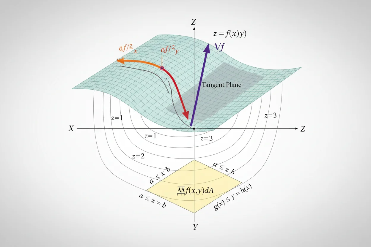
Multivariable calculus extends calculus from functions of one variable to functions involving two or more independent variables. Instead of studying only y = f(x), it considers functions such as z = f(x, y), scalar fields f(x, y, z), and vector-valued mappings between multidimensional spaces. Core ideas include partial derivatives, gradients, directional derivatives, tangent planes, local linear approximation, optimization, multiple integrals, line integrals, and multivariable chain rules. A change in one input can be studied while holding the others fixed, or the combined effect of several simultaneous changes can be represented by vectors and matrices. Integration similarly extends from accumulation over intervals to accumulation over regions, solids, and curves. Multivariable calculus therefore combines the local rate-of-change ideas of derivatives with the geometric and algebraic structure of vectors and matrices. It is used whenever quantities depend on several interacting variables, including geometry, physics, optimization, economics, engineering, probability, and differential equations.
What Is Multivariable Calculus?
Single-variable calculus studies functions such as:
y = f(x)
Multivariable calculus studies functions such as:
z = f(x, y)
or:
w = f(x, y, z)
For example:
f(x, y) = x² + y²
takes two input values and returns one output.
At:
(x, y) = (3, 4)
we have:
f(3, 4) = 3² + 4²
= 9 + 16
= 25
The function can be visualized as a surface:
z = x² + y²
rather than an ordinary two-dimensional curve.
Scalar-Valued Functions of Several Variables
A scalar-valued multivariable function maps several input coordinates to one number.
For example:
T(x, y, z)
might describe temperature at a point in three-dimensional space.
Each input:
(x, y, z)
identifies a position.
The output:
T
is a scalar temperature.
Another example is:
C(x, y)
representing the cost of producing quantities x and y of two products.
Multivariable calculus studies how such outputs change as one or more inputs vary.
Vector-Valued Functions
A multivariable or parameterized function can also produce vectors.
For example:
F(x, y) = (P(x, y), Q(x, y))
assigns a vector to each point in the plane.
Such functions are called vector fields when interpreted geometrically.
A velocity field, force field, or fluid-flow field can all be modeled this way.
Matrices and matrix operations become important when several input and output coordinates interact.
Functions of Two Variables
A common starting point is:
z = f(x, y)
For example:
f(x, y) = 3x² + 2xy − y²
At:
(1, 2)
the value is:
f(1, 2) = 3(1)² + 2(1)(2) − (2)²
= 3 + 4 − 4
= 3
Unlike a one-variable function, infinitely many directions are available from each point in the xy-plane.
This is why multivariable differentiation needs more than one ordinary derivative value.
Graphs of Two-Variable Functions
The graph of:
z = f(x, y)
is generally a surface in three-dimensional space.
For example:
z = x² + y²
is an upward-opening paraboloid.
Each point:
(x, y)
in the domain corresponds to a point:
(x, y, f(x, y))
on the surface.
Geometry becomes central because derivatives can now describe slopes in several directions and tangent objects can become planes rather than lines.
Level Curves
A level curve is obtained by fixing the output:
f(x, y) = c
For:
f(x, y) = x² + y²
the level curves satisfy:
x² + y² = c
For positive c, these are circles of radius:
√c
Level curves provide a two-dimensional representation of a three-dimensional surface.
Contour maps use the same idea to represent elevation, temperature, pressure, and other scalar fields.
Level Surfaces
For a function:
f(x, y, z)
a level surface satisfies:
f(x, y, z) = c
For example:
x² + y² + z² = 25
is a sphere of radius 5.
Level sets allow multivariable functions to be studied geometrically without explicitly plotting an additional output dimension.
They also connect directly with gradients and normal vectors.
Partial Derivatives
A partial derivative measures change with respect to one variable while holding the others constant.
For:
f(x, y)
the two first partial derivatives are:
fₓ = ∂f/∂x
and:
fᵧ = ∂f/∂y
For example, let:
f(x, y) = x²y + 3y²
Differentiate with respect to x while treating y as constant:
fₓ = 2xy
Differentiate with respect to y while treating x as constant:
fᵧ = x² + 6y
These two derivatives describe coordinate-direction slopes.
Partial Derivative Example
For:
f(x, y) = x²y + 3y²
find the partial derivatives at:
(2, 1)
We have:
fₓ = 2xy
so:
fₓ(2, 1) = 2(2)(1)
= 4
Also:
fᵧ = x² + 6y
so:
fᵧ(2, 1) = 4 + 6
= 10
The surface is changing at rate 4 in the positive x-direction and rate 10 in the positive y-direction at that point.
Higher Partial Derivatives
Partial derivatives can themselves be differentiated again.
For f(x, y), second partial derivatives include:
fₓₓ
fᵧᵧ
fₓᵧ
fᵧₓ
For sufficiently smooth functions:
fₓᵧ = fᵧₓ
under familiar continuity conditions on the relevant second partial derivatives.
These second derivatives describe curvature and become important in multivariable optimization.
Gradient
The gradient packages first partial derivatives into a vector.
For:
f(x, y)
the gradient is:
∇f = (fₓ, fᵧ)
For:
f(x, y, z)
it is:
∇f = (fₓ, fᵧ, f_z)
The gradient points in the direction of greatest local increase when it is nonzero.
Its magnitude gives the maximum directional rate of increase per unit distance.
Gradient Example
Let:
f(x, y) = x² + 3xy + y²
Then:
fₓ = 2x + 3y
and:
fᵧ = 3x + 2y
Therefore:
∇f = (2x + 3y, 3x + 2y)
At:
(1, 2)
we get:
∇f(1, 2) = (2 + 6, 3 + 4)
= (8, 7)
So the direction of fastest increase is along:
(8, 7)
after normalization if a unit direction is required.
Directional Derivatives
A partial derivative measures change along a coordinate axis.
A directional derivative measures change in an arbitrary unit direction u.
For a differentiable scalar function:
Dᵤf = ∇f · u
If:
∇f = (8, 7)
and:
u = (3/5, 4/5)
then:
Dᵤf = (8, 7) · (3/5, 4/5)
= 24/5 + 28/5
= 52/5
= 10.4
The dot product converts the gradient into the rate along the selected direction.
Why the Direction Vector Should Be a Unit Vector
If u has length 1, then:
Dᵤf
measures output change per unit distance.
If an arbitrary nonzero vector v is provided, normalize it:
u = v/|v|
For example, if:
v = (3, 4)
then:
|v| = 5
so:
u = (3/5, 4/5)
This keeps directional rates comparable across different directions.
Gradient and Level Curves
At a regular point, the gradient is perpendicular to a level curve:
f(x, y) = c
Suppose t is tangent to the level curve.
Moving along the curve does not change f to first order, so:
Dₜf = 0
But:
Dₜf = ∇f · t
Therefore:
∇f · t = 0
so the gradient is normal to the level curve.
This geometric relationship is fundamental in multivariable calculus.
Tangent Planes
For a differentiable surface:
z = f(x, y)
the tangent plane at:
(a, b, f(a, b))
is:
z − f(a, b) = fₓ(a, b)(x − a) + fᵧ(a, b)(y − b)
This generalizes the tangent-line equation from one-variable calculus.
The tangent plane captures the first-order local behavior of the surface.
Tangent Plane Example
Let:
f(x, y) = x² + y²
Find the tangent plane at:
(1, 2)
First:
f(1, 2) = 1 + 4
= 5
The partial derivatives are:
fₓ = 2x
fᵧ = 2y
So:
fₓ(1, 2) = 2
and:
fᵧ(1, 2) = 4
Therefore:
z − 5 = 2(x − 1) + 4(y − 2)
Simplify:
z = 2x + 4y − 5
This plane approximates the paraboloid near the chosen point.
Multivariable Linear Approximation
The tangent-plane formula gives the multivariable linear approximation:
f(a + Δx, b + Δy)
≈ f(a, b) + fₓ(a, b)Δx + fᵧ(a, b)Δy
Using the gradient:
Δf ≈ ∇f · Δr
where:
Δr = (Δx, Δy)
This is the first-order model of simultaneous input changes.
Linear Approximation Example
Let:
f(x, y) = √(x + y)
near:
(4, 5)
Since:
f(4, 5) = √9 = 3
and:
fₓ = 1/[2√(x + y)]
fᵧ = 1/[2√(x + y)]
we have at (4, 5):
fₓ = fᵧ = 1/6
Estimate:
f(4.06, 4.97)
Here:
Δx = 0.06
Δy = −0.03
So:
Δf ≈ (1/6)(0.06) + (1/6)(−0.03)
= 0.03/6
= 0.005
Therefore:
f(4.06, 4.97) ≈ 3.005
Differentials in Several Variables
For:
z = f(x, y)
the total differential is:
dz = fₓ dx + fᵧ dy
In vector form:
dz = ∇f · dr
This extends the one-variable differentials relationship:
dy = f′(x)dx
to several inputs.
The differential gives the first-order estimated output change produced by small simultaneous input changes.
Multivariable Chain Rule
Suppose:
z = f(x, y)
where both x and y depend on t:
x = x(t)
y = y(t)
Then:
dz/dt = fₓ dx/dt + fᵧ dy/dt
This is a multivariable form of the chain rule.
For example, if:
f(x, y) = x² + y²
then:
dz/dt = 2x dx/dt + 2y dy/dt
The total rate combines the contributions from both changing inputs.
Chain Rule Example
Let:
z = x²y
with:
x = t²
and:
y = t + 1
First:
fₓ = 2xy
and:
fᵧ = x²
Also:
dx/dt = 2t
and:
dy/dt = 1
Therefore:
dz/dt = (2xy)(2t) + x²(1)
Substitute:
x = t²
y = t + 1
giving:
dz/dt = 4t³(t + 1) + t⁴
= 5t⁴ + 4t³
This agrees with differentiating the fully substituted expression directly.
Implicit Differentiation in Several Variables
An equation such as:
F(x, y) = c
defines an implicit curve.
The implicit differentiation formula gives:
dy/dx = −Fₓ/Fᵧ
when:
Fᵧ ≠ 0
The gradient:
∇F = (Fₓ, Fᵧ)
is perpendicular to the same curve.
Thus the implicit derivative and gradient provide complementary descriptions of local geometry.
Critical Points
For a differentiable scalar function:
f(x, y)
an interior critical point commonly occurs where:
∇f = 0
That means:
fₓ = 0
and:
fᵧ = 0
These equations identify candidates for local maxima, minima, or saddle points.
The dedicated optimization framework owns the detailed classification and decision methods.
Critical Point Example
Consider:
f(x, y) = x² + y² − 4x + 6y
Find the gradient:
fₓ = 2x − 4
fᵧ = 2y + 6
Set both equal to zero:
2x − 4 = 0
so:
x = 2
and:
2y + 6 = 0
so:
y = −3
Thus:
(2, −3)
is the critical point.
Completing the square gives:
f(x, y) = (x − 2)² + (y + 3)² − 13
so this point is a global minimum.
Saddle Points
A zero gradient does not always indicate a maximum or minimum.
Consider:
f(x, y) = x² − y²
Then:
∇f = (2x, −2y)
The gradient is zero at:
(0, 0)
But along the x-axis:
f(x, 0) = x² ≥ 0
while along the y-axis:
f(0, y) = −y² ≤ 0
The function rises in some directions and falls in others.
Therefore the point is a saddle point.
Constrained Optimization
Some optimization problems impose a constraint such as:
g(x, y) = c
Rather than allowing movement in every direction, candidate extrema must remain on that constraint.
The gradient of the objective and gradient of the constraint can become parallel at regular constrained extrema:
∇f = λ∇g
This is the foundation of the Lagrange-multiplier method.
The detailed procedure belongs within optimization rather than the general multivariable overview.
Double Integrals
A double integral accumulates a function over a two-dimensional region:
∬ᴿ f(x, y)dA
For a rectangular region:
a ≤ x ≤ b
c ≤ y ≤ d
an iterated form is:
∫ₐᵇ ∫𝚌ᵈ f(x, y)dy dx
when the usual conditions allow it.
If:
f(x, y) ≥ 0
the result can represent volume beneath the surface z = f(x, y).
Double Integral Example
Evaluate:
∬ᴿ (x + y)dA
over:
0 ≤ x ≤ 1
0 ≤ y ≤ 2
Write:
∫₀¹ ∫₀² (x + y)dy dx
Integrate with respect to y:
∫₀² (x + y)dy
= [xy + y²/2]₀²
= 2x + 2
Now integrate with respect to x:
∫₀¹ (2x + 2)dx
= [x² + 2x]₀¹
= 3
Therefore:
∬ᴿ (x + y)dA = 3
Triple Integrals
A triple integral accumulates across a three-dimensional region:
∭ᴱ f(x, y, z)dV
If:
f = 1
then the integral can represent the volume of E.
If:
f = ρ(x, y, z)
is density, then:
∭ᴱ ρ dV
can represent mass.
The same accumulation principle used in one-dimensional integrals extends to higher-dimensional domains.
Iterated Integration
Multiple integrals are often evaluated one variable at a time.
For example:
∫ₐᵇ ∫g₁(x)^g₂(x) f(x, y)dy dx
first treats x as constant while integrating with respect to y.
The resulting expression then becomes a function of x, which is integrated in the outer step.
Understanding which variable is active at each stage prevents confusion.
Line Integrals
A line integral accumulates along a curve rather than over an area.
For a scalar field:
∫꜀ f ds
For a vector field:
∫꜀ F · dr
Parameterization converts the path into a single-variable definite integral.
Line integrals connect multivariable fields with curve geometry and are important in work, circulation, arc length, and potential theory.
Scalar Versus Vector Fields
A scalar field assigns a number to each point:
f(x, y, z)
Examples include temperature and density.
A vector field assigns a vector:
F(x, y, z)
Examples include velocity and force.
Gradients transform scalar fields into vector fields:
f → ∇f
This distinction is important because different differential and integral operators apply to different kinds of fields.
Vector Geometry in Multivariable Calculus
Vectors describe displacement, direction, velocity, normals, tangent directions, and fields.
The dot product measures alignment between vectors.
The cross product provides perpendicular directions and area-related information in three dimensions.
These vector operations make geometric derivative and integral formulas concise.
For example:
Dᵤf = ∇f · u
uses a dot product to extract directional change.
Matrices in Multivariable Calculus
When a function has several inputs and several outputs, derivative information can be organized in a matrix.
For a mapping:
F: Rⁿ → Rᵐ
the derivative matrix contains partial derivatives of each output component with respect to each input variable.
Local changes can then be expressed as:
Δy ≈ AΔx
where A is the derivative matrix.
The calculation uses ordinary matrix multiplication.
Matrix Rank and Local Dimension
The matrix rank of a derivative matrix measures how many independent output directions the local linear model can produce.
If the derivative has full rank, it preserves the maximum possible number of independent directions locally.
If it is rank deficient, some first-order directions collapse.
This rank perspective is important in coordinate transformations, systems of equations, constrained problems, and more advanced multivariable theory.
Coordinate Systems
Cartesian coordinates:
(x, y)
and:
(x, y, z)
are not always the most convenient.
Circular or radial symmetry may suggest polar coordinates:
x = r cos θ
y = r sin θ
Three-dimensional problems may use cylindrical or spherical coordinates.
Changing coordinates can simplify geometry, but the corresponding differential area or volume element must be adjusted appropriately.
Polar Coordinates
In polar coordinates:
x = r cos θ
y = r sin θ
and:
x² + y² = r²
A double-integral area element becomes:
dA = r dr dθ
The extra factor r accounts for how coordinate rectangles in (r, θ) space stretch when mapped into the xy-plane.
This is an example of geometric scaling under a coordinate transformation.
Multivariable Limits
The concept of limits becomes more subtle with several variables.
For:
lim as (x, y) → (a, b) of f(x, y)
the function must approach the same value regardless of the path taken toward (a, b).
Checking one or two paths can disprove a limit if they disagree.
But agreement along a few selected paths does not, by itself, prove the full limit exists.
Path-Dependent Limit Example
Consider:
f(x, y) = x²/(x² + y²)
near:
(0, 0)
Along:
y = 0
we obtain:
f(x, 0) = 1
so the path limit is 1.
Along:
x = 0
we obtain:
f(0, y) = 0
so the path limit is 0.
Because the two paths disagree, the multivariable limit does not exist.
Multivariable Continuity
A function f(x, y) is continuous at:
(a, b)
when:
lim as (x, y) → (a, b) of f(x, y) = f(a, b)
Continuity of common polynomial, exponential, and trigonometric combinations usually allows direct substitution within their domains.
As in one variable, discontinuities and singularities require additional analysis.
Differentiability Is Stronger Than Partial Derivatives
A function can have partial derivatives at a point without being fully differentiable there.
Full differentiability requires one linear map to approximate the function consistently for arbitrary small multidimensional displacements.
When differentiability holds:
Δf = ∇f · Δr + smaller-order error
Partial derivatives along coordinate axes provide necessary information but do not always capture all possible approach directions.
This distinction is uniquely important in several variables.
Multivariable Differential Equations
Multivariable functions also appear in differential equations.
A system can be written:
x′ = F(t, x)
while partial differential equations involve functions of several independent variables and their partial derivatives.
For example, a temperature field:
T(x, y, t)
can vary in two spatial dimensions and time.
Multivariable derivatives describe how it changes separately in each coordinate direction.
Gradient Fields and Potential Functions
If a vector field has form:
F = ∇φ
then φ is a scalar potential function.
Under suitable domain conditions, line integrals of the field become path independent:
∫꜀ F · dr = φ(B) − φ(A)
This relationship connects gradients, directional change, and integration along curves.
It is a higher-dimensional extension of the local-change and accumulation relationship central to calculus.
Multivariable Calculus and the Fundamental Theorem
The Fundamental Theorem Of Calculus connects one-variable derivatives and definite integrals.
Multivariable calculus contains broader versions of the same principle: local derivative information can relate to accumulated quantities over boundaries, curves, surfaces, and regions.
The elementary one-dimensional theorem therefore provides a conceptual model for more advanced integral theorems.
Multivariable Calculus and Linear Transformations
A linear transformation acts exactly through a matrix:
T(x) = Ax
A differentiable nonlinear multivariable mapping behaves approximately like a linear transformation near a point.
The derivative matrix provides that local transformation.
This relationship is one of the strongest conceptual links between multivariable calculus and linear algebra.
Example of Local Matrix Behavior
Suppose:
F(x, y) = (x² + y, xy)
The derivative matrix is formed from partial derivatives:
A = [ 2x 1 ]
[ y x ]
At:
(1, 2)
we obtain:
A = [ 2 1 ]
[ 2 1 ]
For a small displacement:
Δx = (Δx, Δy)
the output change is approximately:
ΔF ≈ AΔx
The matrix has rank 1 at this point, so its local first-order outputs lie along only one independent direction.
Applications of Multivariable Calculus
Multivariable calculus appears whenever several inputs affect an outcome simultaneously.
In physics, fields depend on spatial coordinates and time.
In economics, output or utility may depend on several resources or decisions.
Also, In engineering, temperature, stress, velocity, and pressure vary throughout multidimensional domains.
In probability, joint densities depend on multiple random variables.
In optimization, objectives depend on several decision variables.
The mathematics provides a common language for all of these systems.
Choosing the Right Multivariable Tool
A problem asking how a function changes with one variable while others remain fixed suggests a partial derivative.
A problem asking for the direction of fastest increase suggests a gradient.
A rate along a specified direction suggests a directional derivative.
A local surface estimate suggests a tangent plane or linear approximation.
An interior maximum or minimum suggests optimization.
Accumulation across an area suggests a double integral.
Accumulation along a curve suggests a line integral.
Recognizing the type of question is often more important than memorizing isolated formulas.
Common Multivariable Calculus Mistakes
A common mistake is differentiating every variable when only one partial derivative is requested. For ∂f/∂x, other independent variables are treated as constants.
Another error is assuming partial derivatives alone guarantee full differentiability.
Directional derivatives typically require a unit direction vector.
A zero gradient identifies a critical candidate, not automatically a minimum.
When evaluating multiple integrals, the active integration variable must match the differential and the corresponding bounds.
For multivariable limits, agreement along a few paths does not prove existence, although disagreement along two paths proves nonexistence.
Matrix and vector dimensions should also be checked carefully when derivative information is organized algebraically.
Frequently Asked Questions
What is multivariable calculus?
Multivariable calculus studies differentiation, integration, limits, and optimization for functions involving two or more independent variables.
What is an example of a multivariable function?
f(x, y) = x² + y²
is a function of two variables.
What is a partial derivative?
A partial derivative measures change with respect to one independent variable while holding the others constant.
What is the gradient?
For f(x, y):
∇f = (fₓ, fᵧ)
It points in the direction of greatest local increase when nonzero.
What is a directional derivative?
For unit vector u:
Dᵤf = ∇f · u
It measures the rate of change in the direction u.
What is a tangent plane?
For z = f(x, y), the tangent plane at (a, b) is:
z − f(a, b) = fₓ(a, b)(x − a) + fᵧ(a, b)(y − b)
What is the multivariable linear approximation?
Δf ≈ fₓΔx + fᵧΔy
or:
Δf ≈ ∇f · Δr
How do you find critical points?
For an interior differentiable scalar function, solve:
∇f = 0
Then classify the resulting points with additional analysis.
What is a double integral?
A double integral accumulates a function over a two-dimensional region:
∬ᴿ f(x, y)dA
What is a line integral?
A line integral accumulates a scalar or vector-related quantity along a curve.
Why are multivariable limits harder than one-variable limits?
A point can be approached through infinitely many paths, and the full limit must be independent of the approach path.
How are matrices used in multivariable calculus?
Matrices organize derivative information for mappings with several inputs and outputs and provide the local linear transformation used in first-order approximation.
What does matrix rank mean in multivariable calculus?
The rank of a derivative matrix tells how many independent output directions the local linear model can produce.
What is the difference between multivariable calculus and linear algebra?
Multivariable calculus studies change and accumulation in several variables. Linear algebra studies vectors, matrices, linear systems, and linear transformations. The subjects meet when derivatives of multivariable mappings are represented by vectors and matrices.




