


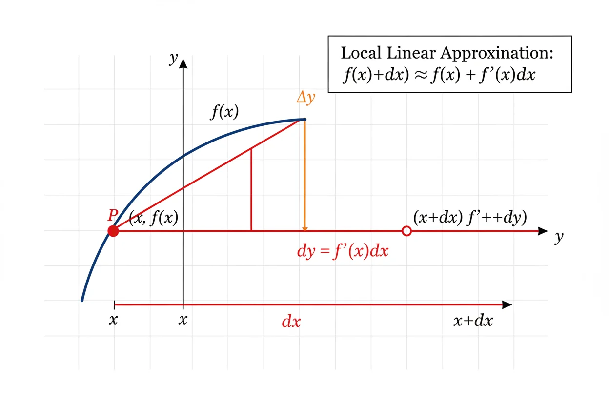
Differentials describe how a small change in an input produces an estimated change in the output of a differentiable function. If y = f(x), the differential of x is written dx, while the corresponding differential of y is dy = f′(x) dx. The quantity dy uses the tangent-line slope to approximate the actual change Δy when dx is small. Differentials therefore provide a compact way to express local linear behavior, propagate measurement changes, and estimate how sensitive one quantity is to another. They are closely connected to the derivative, but dx and dy play a distinct role from the derivative ratio dy/dx. For sufficiently small input changes, dy is usually close to Δy, although the two are not generally identical. The approximation becomes less reliable as the input change becomes larger or the function bends more strongly. Understanding differentials is useful in approximation, error analysis, related rates, integration notation, and multivariable calculus.
What Are Differentials?
Suppose:
y = f(x)
The differential of the independent variable is written:
dx
The differential of y is defined by:
dy = f′(x) dx
This formula states that the local change predicted by the tangent line equals the derivative multiplied by a chosen small input change.
For example, if:
y = x²
then:
dy = 2x dx
At x = 3, if:
dx = 0.02
then:
dy = 2(3)(0.02)
dy = 0.12
So increasing x from 3 by 0.02 produces an estimated change in y of 0.12.
Differential Formula
The central formula is:
dy = f′(x) dx
where:
- dx represents a change in the independent variable,
- f′(x) is the local rate of change,
- dy is the resulting linearized change in the dependent variable.
Dividing formally by dx gives:
dy/dx = f′(x)
This is the familiar derivative notation.
The wider theory of derivatives develops rates of change in several forms, while differentials emphasize how those rates translate a small input change into a corresponding output change.
Differential Versus Actual Change
The actual change in a function is:
Δy = f(x + Δx) − f(x)
If we identify the small input increment with:
dx = Δx
then the differential is:
dy = f′(x)Δx
For small Δx:
Δy ≈ dy
This is an approximation, not an exact equality in general.
Consider again:
f(x) = x²
at:
x = 3
with:
dx = 0.02
The differential is:
dy = 2(3)(0.02) = 0.12
The actual change is:
Δy = (3.02)² − 3²
= 9.1204 − 9
= 0.1204
Therefore:
dy = 0.12
while:
Δy = 0.1204
The differential is close because the input change is small.
Why Differentials Work
A differentiable function looks increasingly like its tangent line when viewed sufficiently close to a point.
Near x = a:
f(a + dx) ≈ f(a) + f′(a)dx
Because:
dy = f′(a)dx
we can write:
f(a + dx) ≈ f(a) + dy
This is the basic idea behind linear approximation.
The closer the function behaves to a straight line over the chosen interval, the better the differential usually approximates the true change.
How to Find a Differential
Suppose:
y = f(x)
First find the derivative f′(x). Then multiply it by dx.
For:
y = x³ + 2x
differentiate:
f′(x) = 3x² + 2
Therefore:
dy = (3x² + 2)dx
At:
x = 2
and:
dx = 0.01
we get:
dy = 3(2²) + 2
= (12 + 2)(0.01)
= 0.14
So the predicted output change is 0.14.
Example: Estimate a Square Root
Differentials can approximate difficult numerical values.
Let:
y = √x
Suppose we want to estimate:
√25.4
Choose the nearby easy value:
x = 25
Then:
y = √25 = 5
The input change is:
dx = 0.4
Differentiate:
dy = 1/(2√x) dx
At x = 25:
dy = 1/(2·5)(0.4)
= 0.04
Therefore:
√25.4 ≈ 5 + 0.04
√25.4 ≈ 5.04
The actual value is approximately 5.03984, so the differential produces a close estimate.
Example: Estimate a Cube
Suppose:
y = x³
and we want to estimate:
2.01³
Start with:
x = 2
and:
dx = 0.01
Since:
dy = 3x² dx
we obtain:
dy = 3(2²)(0.01)
= 12(0.01)
= 0.12
Because:
2³ = 8
the estimate is:
2.01³ ≈ 8 + 0.12
≈ 8.12
The exact value is:
2.01³ = 8.120601
Again, the differential captures most of the change.
Constant Rule for Differentials
If:
y = c
where c is constant, then:
dy = 0
because:
d/dx[c] = 0
A constant output does not change when x changes.
Power Rule for Differentials
If:
y = xⁿ
then:
dy = nxⁿ⁻¹ dx
For example:
y = x⁵
gives:
dy = 5x⁴ dx
At x = 2 and dx = 0.1:
dy = 5(2⁴)(0.1)
= 5(16)(0.1)
= 8
The differential predicts an output increase of 8 for that local input change.
Sum and Difference Rules
If:
y = f(x) + g(x)
then:
dy = [f′(x) + g′(x)]dx
Similarly, if:
y = f(x) − g(x)
then:
dy = [f′(x) − g′(x)]dx
For example:
y = x³ + 4x² − 2x
gives:
dy = (3x² + 8x − 2)dx
The same differentiation rules that produce derivatives determine the corresponding differentials.
Product Differentials
If:
y = u(x)v(x)
then the differential is:
dy = [u′(x)v(x) + u(x)v′(x)]dx
Equivalently, using differential notation:
d(uv) = u dv + v du
This follows from the usual product differentiation rule.
For example, if:
y = x²eˣ
then:
dy = [2xeˣ + x²eˣ]dx
dy = eˣ(2x + x²)dx
Quotient Differentials
For:
y = u/v
with v ≠ 0:
d(u/v) = (v du − u dv)/v²
If u and v both depend on x, this is equivalent to applying the quotient differentiation rule and then multiplying by dx.
Differential notation can therefore make familiar differentiation identities more compact.
Differentials of Composite Functions
Suppose:
y = f(u)
and:
u = g(x)
Then:
dy = f′(u)du
while:
du = g′(x)dx
Substituting gives:
dy = f′(g(x))g′(x)dx
This is the differential form of the chain rule.
For example:
y = (x² + 1)⁴
Let:
u = x² + 1
Then:
dy = 4u³ du
and:
du = 2x dx
Therefore:
dy = 8x(x² + 1)³ dx
Relative Change
Differentials can express approximate relative change.
For y ≠ 0:
dy/y
represents the differential relative to the current output value.
Multiplying by 100 gives an approximate percentage change:
percentage change ≈ 100(dy/y)%
For:
y = x²
we have:
dy = 2x dx
so:
dy/y = 2x dx/x²
= 2dx/x
Thus a small relative change in x produces approximately twice that relative change in x².
If x rises by approximately 1%, x² rises by approximately 2%, provided the change is sufficiently small.
Differentials and Measurement Error
Suppose a measured quantity x has possible error:
dx
and:
y = f(x)
Then the resulting approximate error in y is:
dy = f′(x)dx
This is useful because measurement uncertainty in one quantity often propagates into calculations based on that quantity.
Consider the area of a circle:
A = πr²
Its differential is:
dA = 2πr dr
If:
r = 10 cm
and the radius may be off by:
dr = 0.02 cm
then:
dA = 2π(10)(0.02)
dA = 0.4π
dA ≈ 1.257 cm²
So the resulting area error is approximately 1.257 cm² in magnitude.
Relative Error Example
For a circle:
A = πr²
we found:
dA = 2πr dr
Divide by A:
dA/A = 2πr dr/(πr²)
Simplify:
dA/A = 2dr/r
This means the relative area error is approximately twice the relative radius error.
If the radius measurement has approximately 0.5% relative error, the corresponding area has approximately:
2(0.5%) = 1%
relative error.
Differentials and Related Rates
Differentials and rates are closely connected.
If:
y = f(x)
then:
dy = f′(x)dx
Dividing changes by a time differential dt gives:
dy/dt = f′(x) dx/dt
This structure appears naturally in related rates problems.
For example, from:
A = πr²
we obtain:
dA/dt = 2πr dr/dt
The geometry provides the relationship, while differentiation connects the rates.
Differentials in Several Variables
If a function depends on multiple variables, its differential includes contributions from each independent input.
For:
z = f(x, y)
the total differential is:
dz = (∂f/∂x)dx + (∂f/∂y)dy
The quantities ∂f/∂x and ∂f/∂y are obtained using a partial derivative with respect to each variable.
For example:
z = x²y + y³
Then:
∂z/∂x = 2xy
and:
∂z/∂y = x² + 3y²
Therefore:
dz = 2xy dx + (x² + 3y²)dy
This estimates how z changes when both x and y change slightly.
Multivariable Differential Example
Let:
z = x² + 3xy + y²
At:
x = 2
y = 1
suppose:
dx = 0.01
dy = −0.02
Find the partial derivatives:
∂z/∂x = 2x + 3y
At (2, 1):
∂z/∂x = 4 + 3 = 7
Also:
∂z/∂y = 3x + 2y
At (2, 1):
∂z/∂y = 6 + 2 = 8
So:
dz = 7(0.01) + 8(−0.02)
= 0.07 − 0.16
= −0.09
The total differential predicts that z decreases by approximately 0.09.
These ideas belong naturally to multivariable calculus, where several independent inputs may vary simultaneously.
Differential Versus Directional Derivative
A total differential estimates the change caused by a small displacement in the input variables.
A directional derivative instead measures the rate of change per unit distance in one specified direction.
For a differentiable function f(x, y), both concepts depend on local derivative information, but they answer different questions.
The differential asks approximately how much the output changes for a particular small displacement. The directional derivative asks how quickly the function changes when moving in a chosen direction.
Differentials and the Dot Product
In several variables, total differentials have a vector interpretation.
For:
f(x, y)
the gradient is:
∇f = (fₓ, fᵧ)
and the displacement can be written:
dr = (dx, dy)
Then:
df = ∇f · dr
The symbol · is the dot product.
This expresses the total differential as the component of local gradient information acting along the chosen displacement.
Differentials in Differential Equations
Differential notation is also widely used in differential equations.
For example:
dy/dx = xy
can be rearranged in a separable setting as:
(1/y)dy = x dx
Integrating both sides gives:
ln|y| = x²/2 + C
Differential notation makes the separation structure easy to see.
However, symbols such as dx and dy should not be rearranged mechanically in every equation. The manipulation must correspond to a mathematically valid transformation.
Differentials and Integration
The notation:
∫ f(x) dx
uses dx to indicate the variable with respect to which integration occurs.
For example:
∫ x² dx
means integration with respect to x.
The connection between differentiation and integration becomes especially clear when:
dy = f′(x)dx
is integrated:
∫ dy = ∫ f′(x)dx
giving:
y = f(x) + C
A definite integral uses the same differential notation while accumulating across fixed limits.
When Is the Differential Approximation Accurate?
The approximation:
Δy ≈ dy
is generally strongest when dx is small and the function is differentiable with limited curvature near the point.
For a perfectly linear function:
f(x) = mx + b
the approximation becomes exact because:
Δy = mΔx
and:
dy = m dx
If:
dx = Δx
then:
Δy = dy
For nonlinear functions, curvature creates the difference between the tangent-line prediction and the actual change.
How Error Changes With dx
Consider:
f(x) = x²
The exact change is:
Δy = (x + dx)² − x²
Expand:
Δy = 2x dx + (dx)²
The differential is:
dy = 2x dx
Therefore:
Δy − dy = (dx)²
The omitted term is second order in dx.
As dx becomes very small, (dx)² becomes even smaller relative to dx. This helps explain why differentials provide effective local approximations.
Differentiability and Differentials
A standard total differential requires differentiability.
Differentiability implies continuity at the point, although continuity alone does not guarantee differentiability.
At a sharp corner, for example, a single tangent slope may not exist. Without an appropriate derivative, the ordinary one-variable differential:
dy = f′(x)dx
cannot be formed there in the usual way.
Common Mistakes With Differentials
A common error is assuming:
dy = Δy
for every finite change.
In general:
dy ≈ Δy
when the change is sufficiently small. Exact equality occurs for linear functions and in certain special circumstances.
Another mistake is forgetting to evaluate the derivative at the specified point before multiplying by dx.
It is also important to distinguish:
dx
from:
dy/dx
The first represents an input differential, while the second represents a derivative.
In multivariable problems, every changing independent variable must be included in the total differential. Ignoring a term such as fᵧdy can produce an incorrect estimate.
Finally, the sign matters. A negative differential indicates that the local linear estimate predicts a decrease in the output, not merely an error magnitude.
Frequently Asked Questions
What are differentials in calculus?
Differentials describe local changes in variables. If y = f(x), then:
dy = f′(x)dx
relates a small input change dx to the corresponding linearized output change dy.
What is the main differential formula?
For a differentiable function y = f(x):
dy = f′(x)dx
What is the difference between dy and Δy?
Δy is the actual change:
Δy = f(x + Δx) − f(x)
while dy is the tangent-line estimate:
dy = f′(x)dx
When dx = Δx and the change is small:
Δy ≈ dy
Is dx always very small?
Differential methods are most useful when dx is small enough for a local linear approximation to be accurate. The notation itself does not assign a fixed numerical size to dx.
When does dy equal Δy exactly?
For a linear function, dy equals Δy whenever dx = Δx. For nonlinear functions, the values generally differ.
How are differentials used for approximation?
Use:
f(x + dx) ≈ f(x) + f′(x)dx
The term f′(x)dx is the differential dy.
How are differentials used in error analysis?
If x has a small measurement error dx, then:
dy = f′(x)dx
approximates the resulting error in y = f(x).
What is a total differential?
For a function of several variables, such as z = f(x, y):
dz = fₓ dx + fᵧ dy
It estimates the combined change caused by small changes in both independent variables.
Are differentials the same as derivatives?
No. A derivative is a rate such as dy/dx. A differential such as dy represents the local output change obtained by multiplying that rate by dx.
Why does dx appear in an integral?
In an integral such as ∫ f(x) dx, dx identifies the variable of integration and fits naturally with the differential relationship between integration and differentiation.
What makes a differential approximation inaccurate?
Large input changes, strong curvature, nondifferentiability, and evaluation near problematic domain points can all reduce the accuracy of the linear approximation.




