


Derivatives describe how functions change. A derivative can measure the slope of a curve, instantaneous velocity, acceleration, growth, decline, marginal change, sensitivity, or another rate that depends on an input variable. For a function f(x), common derivative notation includes f′(x), y′, dy/dx, and d/dx[f(x)]. The first derivative describes the immediate rate of change, while second and higher derivatives describe how that rate itself changes. Different mathematical situations also lead to partial derivatives, directional derivatives, implicit derivatives, and other specialized forms. The basic derivative comes from a limiting difference quotient, but most practical calculations use established differentiation rules. Understanding derivatives therefore involves more than finding a slope: it includes interpreting signs, units, higher-order behavior, critical points, and how different derivative forms apply to different kinds of functions.
What Are Derivatives?
Derivatives are mathematical quantities that measure rates of change.
If:
y = f(x)
then the first derivative can be written:
f′(x)
or:
dy/dx
The detailed calculation of an individual derivative begins with the limit definition:
f′(x) = lim [f(x + h) − f(x)]/h as h → 0
The expression before the limit measures average change over a small interval. Allowing h to approach zero gives the instantaneous rate of change when the limit exists.
Derivatives can themselves be functions. Once f′(x) is known, it can be evaluated at different inputs to determine how the original function changes throughout its domain.
Basic Derivative Example
Consider:
f(x) = x³ − 4x² + 5x
Differentiate term by term:
f′(x) = 3x² − 8x + 5
At x = 2:
f′(2) = 3(2²) − 8(2) + 5
= 12 − 16 + 5
= 1
Therefore, the instantaneous rate of change of f at x = 2 is:
1
Geometrically, the tangent line to the graph has slope 1 at that point.
First Derivatives
The first derivative measures the immediate rate at which one quantity changes with respect to another.
For:
f(x) = x²
the first derivative is:
f′(x) = 2x
At x = 1:
f′(1) = 2
At x = 4:
f′(4) = 8
The changing derivative values show that the slope of x² becomes steeper as x increases on the positive side.
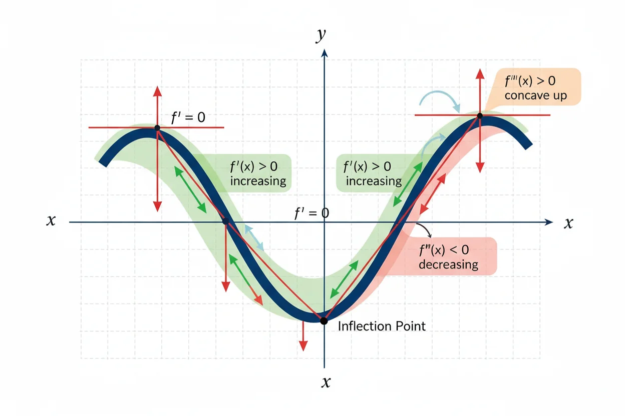
If f′(x) is positive on an interval, f is increasing there. If it is negative, f is decreasing there.
Second Derivatives
The second derivative differentiates the first derivative.
It can be written:
f″(x)
or:
d²y/dx²
If:
f(x) = x³
then:
f′(x) = 3x²
and:
f″(x) = 6x
The second derivative measures how the first derivative changes.
In a motion problem, if position is s(t), then:
s′(t) = velocity
and:
s″(t) = acceleration
The second derivative also plays an important role in analyzing curvature and concavity.
Higher-Order Derivatives
The process can continue beyond the second derivative.
The third derivative is:
f‴(x)
and the nth derivative may be written:
f⁽ⁿ⁾(x)
For example:
f(x) = x⁴
Then:
f′(x) = 4x³
f″(x) = 12x²
f‴(x) = 24x
f⁽⁴⁾(x) = 24
f⁽⁵⁾(x) = 0
Higher-order derivatives are useful whenever changes in lower-order rates matter.
Common Derivative Rules
Many derivatives can be calculated without returning to the limit definition each time.
Constant Rule
For a constant c:
d/dx[c] = 0
For example:
d/dx[12] = 0
Power Rule
For:
f(x) = xⁿ
the power rule gives:
f′(x) = nxⁿ⁻¹
For example:
d/dx[x⁷] = 7x⁶
Constant Multiple Rule
For constant c:
d/dx[c f(x)] = c f′(x)
For example:
d/dx[5x⁴] = 20x³
Sum Rule
d/dx[f(x) + g(x)] = f′(x) + g′(x)
Difference Rule
d/dx[f(x) − g(x)] = f′(x) − g′(x)
These rules allow polynomial expressions to be differentiated term by term.
Derivatives of Products
When two functions are multiplied, the product rule applies:
d/dx[f(x)g(x)] = f′(x)g(x) + f(x)g′(x)
Consider:
y = x²eˣ
Then:
y′ = 2xeˣ + x²eˣ
Factor:
y′ = eˣ(2x + x²)
Simply multiplying the individual derivatives would not give the correct answer.
Derivatives of Quotients
For:
y = f(x)/g(x)
the quotient rule is:
y′ = [g(x)f′(x) − f(x)g′(x)]/[g(x)]²
provided:
g(x) ≠ 0
For example:
y = x/(x + 1)
Then:
y′ = [(x + 1)(1) − x(1)]/(x + 1)²
= 1/(x + 1)²
Derivatives of Composite Functions
If one function is placed inside another, the chain rule is usually required.
Suppose:
y = (3x² + 1)⁴
Differentiate the outer power first:
4(3x² + 1)³
Then multiply by the derivative of the inner function:
6x
Therefore:
y′ = 24x(3x² + 1)³
The inner derivative is essential.
Exponential Derivatives
For the natural exponential function:
d/dx[eˣ] = eˣ
More generally, for a positive constant a:
d/dx[aˣ] = aˣ ln(a)
For example:
d/dx[5ˣ] = 5ˣ ln(5)
If the exponent is itself a function, the chain rule may also be needed.
Logarithmic Derivatives
A fundamental logarithmic derivative is:
d/dx[ln x] = 1/x
for:
x > 0
For example:
d/dx[4ln x] = 4/x
For a composite logarithm:
y = ln(x² + 1)
the derivative is:
y′ = 2x/(x² + 1)
Trigonometric Derivatives
Important trigonometric derivatives include:
d/dx[sin x] = cos x
d/dx[cos x] = −sin x
d/dx[tan x] = sec²x
For example:
f(x) = 3sin x + 2cos x
Then:
f′(x) = 3cos x − 2sin x
These standard formulas assume angles are measured in radians.
Implicit Derivatives
Sometimes x and y are connected by an equation that is not solved explicitly for y.
Consider:
x² + y² = 25
Differentiate both sides with respect to x:
2x + 2y(dy/dx) = 0
Solve:
2y(dy/dx) = −2x
dy/dx = −x/y
This process is called implicit differentiation.
It is especially useful for circles, algebraic curves, and relationships where isolating y would create unnecessary complexity.
Partial Derivatives
When a function depends on several independent variables, its rate of change can be examined one variable at a time.
Suppose:
f(x, y) = x²y + 4xy²
Holding y constant and differentiating with respect to x gives:
∂f/∂x = 2xy + 4y²
Holding x constant and differentiating with respect to y gives:
∂f/∂y = x² + 8xy
These are partial derivatives.
They form an important bridge between single-variable calculus and multivariable analysis.
Directional Derivatives
A partial derivative measures change along a coordinate direction. A directional derivative measures change in a chosen direction.
For a differentiable scalar function f and unit vector u, the directional derivative can be expressed as:
Dᵤf = ∇f · u
The symbol ∇f represents the gradient.
This combines differentiation with the dot product to measure the component of the gradient in a selected direction.
Derivatives and Differentials
If:
y = f(x)
then a differential relationship can be written:
dy = f′(x) dx
The quantities dx and dy are differentials that describe a local linear relationship between small changes.
For a small change Δx:
Δy ≈ f′(x)Δx
This approximation becomes useful when a full function evaluation is inconvenient but a nearby derivative is known.
Positive and Negative Derivatives
The sign of a derivative contains useful information about function behavior.
If:
f′(x) > 0
the function is locally increasing.
If:
f′(x) < 0
the function is locally decreasing.
If:
f′(x) = 0
the function has a horizontal tangent at that point, assuming the derivative exists.
A zero derivative does not automatically prove that a point is a maximum or minimum. The behavior on either side must also be considered.
Critical Points
A critical number usually occurs where:
f′(x) = 0
or where f′(x) does not exist while f itself is defined.
Consider:
f(x) = x² − 6x + 10
Differentiate:
f′(x) = 2x − 6
Set the derivative equal to zero:
2x − 6 = 0
x = 3
This identifies a critical point.
Derivative-based optimization uses such points to locate possible maxima and minima.
Second Derivative and Concavity
The second derivative helps describe how a graph bends.
If:
f″(x) > 0
the graph is concave upward locally.
If:
f″(x) < 0
the graph is concave downward locally.
Consider:
f(x) = x³ − 3x²
Then:
f′(x) = 3x² − 6x
and:
f″(x) = 6x − 6
The sign of f″ changes at:
x = 1
This may indicate an inflection point if the concavity actually changes across that value.
Derivatives in Motion
If position is:
s(t)
then the first derivative gives velocity:
v(t) = s′(t)
and the second derivative gives acceleration:
a(t) = s″(t)
Suppose:
s(t) = 2t³ − 3t² + 4t
Then:
v(t) = 6t² − 6t + 4
and:
a(t) = 12t − 6
At t = 2:
v(2) = 6(4) − 12 + 4 = 16
a(2) = 24 − 6 = 18
If position is measured in meters and time in seconds, the velocity is 16 m/s and acceleration is 18 m/s².
Derivatives and Related Rates
When several changing quantities are connected by an equation, differentiation can relate their rates.
For a sphere:
V = (4/3)πr³
Differentiate with respect to time:
dV/dt = 4πr² dr/dt
This equation connects the rate of volume change to the rate of radius change.
Such problems form the basis of related rates.
Derivatives and Continuity
Differentiability requires continuity at the point being differentiated.
Therefore:
differentiable ⇒ continuous
The reverse does not necessarily hold.
For example:
f(x) = |x|
is continuous at x = 0, but its left-hand slope is −1 and its right-hand slope is 1.
Because those slopes differ:
f′(0) does not exist
A continuous function can therefore fail to be differentiable.
Derivatives and Integrals
Differentiation measures local change, while integration accumulates change.
A definite integral connects to derivatives through:
∫ₐᵇ f(x) dx = F(b) − F(a)
where:
F′(x) = f(x)
The Fundamental Theorem of Calculus formalizes the inverse relationship between these two central calculus operations.
Derivatives in Differential Equations
A differential equation contains an unknown function together with one or more of its derivatives.
For example:
dy/dx = 2y
states that the derivative of y is always twice the current value of y.
Differentiation normally begins with a known function and finds its rate of change. Differential equations reverse the perspective by specifying derivative relationships and asking which functions satisfy them.
Derivatives in Several Dimensions
In several variables, derivatives take forms that reflect different directions and structures.
Partial derivatives measure coordinate-wise change. The gradient combines first partial derivatives into a vector. Directional derivatives measure rates along chosen directions.
These concepts belong naturally to the broader Calculus & Linear Algebra framework because multivariable change frequently interacts with vector and matrix methods.
A cross product is not itself a derivative, but vector derivatives and cross products can appear together in more advanced three-dimensional analysis.
When Derivatives Do Not Exist
Not every function is differentiable at every point in its domain.
A derivative may fail to exist at:
- a discontinuity,
- a sharp corner,
- a cusp,
- a vertical tangent,
- or another point where the limiting slope is not a single finite number.
For example:
f(x) = |x|
has a corner at x = 0.
For:
f(x) = x¹ᐟ³
the derivative is:
f′(x) = 1/(3x²ᐟ³)
which becomes unbounded as x approaches 0.
The function remains defined at 0, but the ordinary finite derivative there does not exist.
Units of Derivatives
A derivative has units equal to:
units of output / units of input
If distance is measured in kilometers and time in hours:
ds/dt
has units of kilometers per hour.
If revenue R depends on quantity q:
dR/dq
has units of currency per unit.
Units often reveal the practical meaning of a derivative more clearly than the formula alone.
Common Mistakes With Derivatives
A frequent mistake is confusing a function value with its derivative value. The statement f(3) = 10 says nothing by itself about f′(3).
Another error is applying the power rule incorrectly. For:
x⁶
the derivative is:
6x⁵
not 6x⁶.
Products, quotients, and composite functions also require their appropriate rules. Differentiating their components independently and simply combining the results usually fails.
It is also important not to assume that every point on a continuous graph has a derivative. Corners and other nonsmooth points provide common counterexamples.
Finally, derivatives should be interpreted with units and context. A derivative of 5 might mean 5 meters per second, 5 dollars per unit, 5 degrees per hour, or something entirely different depending on the variables involved.
Frequently Asked Questions
What are derivatives in mathematics?
Derivatives are quantities that measure instantaneous rates of change. Geometrically, a first derivative gives the slope of a tangent line to a graph.
What is the basic derivative formula?
The first-principles definition is:
f′(x) = lim [f(x + h) − f(x)]/h as h → 0
when this limit exists.
What is the difference between first and second derivatives?
The first derivative measures how the original function changes. The second derivative measures how the first derivative changes.
What does a positive derivative mean?
It generally means the function is increasing locally.
What does a negative derivative mean?
It generally means the function is decreasing locally.
What does a derivative of zero mean?
It means the tangent line is horizontal at that point. The point may be a local maximum, local minimum, or another stationary point.
Are derivatives always functions?
When differentiation produces a rule valid over part of a domain, that rule is a derivative function. A derivative can also be evaluated at one specific point to produce a numerical value.
Can derivatives be taken more than once?
Yes. A function can have second, third, and higher-order derivatives whenever the required differentiability conditions hold.
What is the difference between partial and ordinary derivatives?
An ordinary derivative typically involves a function of one independent variable. A partial derivative measures change with respect to one variable while holding the other independent variables constant.
Can a continuous function have no derivative?
Yes. Continuity does not guarantee differentiability. The function |x| is continuous at 0 but has no derivative there.
How are derivatives related to integrals?
Derivatives measure local change, while integrals accumulate quantities. Under suitable conditions, differentiation and integration are inverse processes.
Why are derivatives useful?
They allow changing systems to be analyzed quantitatively. Applications include motion, optimization, economics, engineering, probability, physical models, approximation, and differential equations.




