


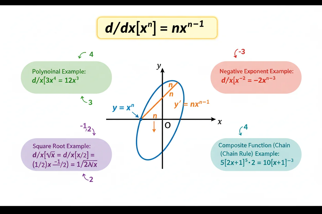
The power rule is a differentiation formula for functions containing powers of the variable. If f(x) = xⁿ, then f′(x) = nxⁿ⁻¹ wherever the power function is differentiable. The rule says to multiply by the exponent and then reduce the exponent by one. It works directly for positive integer powers, negative integer powers, and many fractional or real powers on appropriate domains. Constant coefficients remain in front, so d/dx[cxⁿ] = cnxⁿ⁻¹. Polynomial derivatives can therefore be found by applying the power rule term by term. When a power contains a nontrivial inner function, such as (3x + 1)⁵, the power rule must be combined with the chain rule. Products and quotients can also require their own differentiation rules rather than applying the power rule to the entire expression. The power rule is one of the most frequently used tools in differential calculus because it turns many derivative calculations into simple algebra.
What Is the Power Rule?
For a power function:
f(x) = xⁿ
the power rule states:
f′(x) = nxⁿ⁻¹
where the formula is applied on points where the corresponding real power function is differentiable.
The procedure is:
bring the exponent down as a coefficient
then:
subtract 1 from the exponent
For example:
d/dx[x⁵] = 5x⁴
The original exponent:
5
becomes the coefficient, and the new exponent is:
5 − 1 = 4
Power Rule Formula
The standard formula is:
d/dx[xⁿ] = nxⁿ⁻¹
For a constant coefficient c:
d/dx[cxⁿ] = cnxⁿ⁻¹
For example:
d/dx[7x⁴]
= 7(4)x³
= 28x³
This follows from the constant-multiple rule for derivatives.
Basic Power Rule Examples
Differentiate:
f(x) = x³
Apply the formula:
f′(x) = 3x²
For:
f(x) = x⁸
we get:
f′(x) = 8x⁷
For:
f(x) = x
write:
x = x¹
Then:
d/dx[x] = 1x⁰
= 1
The same formula covers the basic derivative of x.
Power Rule With a Constant Coefficient
Differentiate:
f(x) = 6x⁵
The exponent is:
5
Multiply the coefficient by 5:
6 × 5 = 30
Reduce the exponent:
5 − 1 = 4
Therefore:
f′(x) = 30x⁴
For:
f(x) = −3x⁷
we get:
f′(x) = −21x⁶
The sign and original coefficient remain part of the multiplication.
Power Rule for a Constant
A constant can be viewed as:
c = cx⁰
Applying the power rule formally:
d/dx[cx⁰] = c(0)x⁻¹
= 0
Therefore:
d/dx[c] = 0
For example:
d/dx[12] = 0
This agrees with the geometric fact that a horizontal line has zero slope.
Differentiating a Polynomial
Consider:
f(x) = 4x⁵ − 3x³ + 2x² − 7x + 9
Apply the power rule term by term:
d/dx[4x⁵] = 20x⁴
d/dx[−3x³] = −9x²
d/dx[2x²] = 4x
d/dx[−7x] = −7
d/dx[9] = 0
Therefore:
f′(x) = 20x⁴ − 9x² + 4x − 7
This term-by-term procedure is one reason polynomial derivatives are straightforward.
Negative Exponents
The power rule also works for negative integer powers where the function is defined.
Consider:
f(x) = x⁻³
Then:
f′(x) = −3x⁻⁴
Rewrite:
f′(x) = −3/x⁴
The original function:
1/x³
is undefined at:
x = 0
so its derivative formula applies on intervals where:
x ≠ 0
Reciprocal Example
Differentiate:
f(x) = 1/x
Rewrite:
f(x) = x⁻¹
Apply the power rule:
f′(x) = −1x⁻²
Therefore:
f′(x) = −1/x²
for:
x ≠ 0
Rewriting reciprocals as negative powers can often eliminate the need for a more complicated rule.
Fractional Exponents
Radicals can often be rewritten as fractional powers.
For example:
√x = x¹ᐟ²
Differentiate:
d/dx[x¹ᐟ²]
= 1/2 x⁻¹ᐟ²
Therefore:
d/dx[√x] = 1/(2√x)
for:
x > 0
The original function is defined at x = 0, but this derivative formula becomes unbounded there, and √x does not have a finite ordinary derivative at zero.
Cube Root Example
Write:
∛x = x¹ᐟ³
Then:
d/dx[x¹ᐟ³]
= 1/3 x⁻²ᐟ³
So:
d/dx[∛x] = 1/(3x²ᐟ³)
for:
x ≠ 0
At:
x = 0
the derivative is not finite.
Fractional exponents therefore require attention to both the function’s real domain and the derivative’s domain.
Fractional Power With a Coefficient
Differentiate:
f(x) = 8x³ᐟ²
Apply the power rule:
f′(x) = 8(3/2)x¹ᐟ²
= 12x¹ᐟ²
Therefore:
f′(x) = 12√x
on the real domain where the original expression is defined.
Evaluating a Derivative at a Point
Suppose:
f(x) = 3x⁴
Then:
f′(x) = 12x³
At:
x = 2
the derivative is:
f′(2) = 12(2³)
= 12(8)
= 96
This is the instantaneous slope of the function at x = 2.
The broader derivative concept explains this rate-of-change interpretation.
Tangent Line Using the Power Rule
Find the tangent line to:
f(x) = x³
at:
x = 2
First find the point:
f(2) = 8
Then calculate the derivative:
f′(x) = 3x²
At x = 2:
f′(2) = 12
So the tangent slope is:
m = 12
Using point-slope form:
y − 8 = 12(x − 2)
Therefore:
y = 12x − 16
The power rule supplies the slope needed for the tangent line.
Power Rule and the Limit Definition
The limit definition of a derivative is:
f′(x) = lim [f(x+h) − f(x)]/h as h → 0
For:
f(x) = x²
substitute:
f′(x) = lim [(x+h)² − x²]/h
Expand:
= lim [x² + 2xh + h² − x²]/h
Simplify:
= lim [2xh + h²]/h
For h ≠ 0:
= lim (2x + h)
As h → 0:
f′(x) = 2x
This agrees with the power rule:
d/dx[x²] = 2x
The rule is therefore a shortcut supported by the derivative’s limiting definition.
Why the Exponent Drops by One
For positive integer powers, the pattern follows from expanding:
(x + h)ⁿ
in the difference quotient.
After subtracting xⁿ, every remaining term contains h.
Dividing by h leaves a leading term:
nxⁿ⁻¹
while all terms containing additional powers of h vanish as:
h → 0
The result is:
d/dx[xⁿ] = nxⁿ⁻¹
This provides a conceptual reason for both parts of the rule.
Power Rule and the Chain Rule
The direct power rule applies immediately to:
xⁿ
But if the base is a function of x:
[g(x)]ⁿ
the chain rule is also required:
d/dx[g(x)]ⁿ = n[g(x)]ⁿ⁻¹g′(x)
For example:
f(x) = (3x + 1)⁵
The outer power derivative is:
5(3x + 1)⁴
The derivative of the inner function is:
3
Therefore:
f′(x) = 15(3x + 1)⁴
Composite Power Example
Differentiate:
f(x) = (x² + 4)³
Apply the outer power rule:
3(x² + 4)²
Then differentiate the inside:
d/dx[x² + 4] = 2x
Multiply:
f′(x) = 6x(x² + 4)²
Writing only:
3(x² + 4)²
would miss the inner derivative and therefore be incomplete.
Power Rule and the Product Rule
The power rule does not replace the product rule.
Consider:
f(x) = x²eˣ
The function is a product of:
x²
and:
eˣ
Differentiate:
f′(x) = (2x)eˣ + x²eˣ
Therefore:
f′(x) = eˣ(x² + 2x)
The power rule handles x², while the product rule combines the derivatives of the two factors.
Product of Two Powers
Sometimes an apparent product can be simplified before differentiating.
Consider:
f(x) = x³x⁵
Combine powers:
x³x⁵ = x⁸
Then:
f′(x) = 8x⁷
Using the product rule would also work:
f′(x) = 3x²x⁵ + x³5x⁴
= 3x⁷ + 5x⁷
= 8x⁷
Simplifying first is usually faster.
Power Rule and the Quotient Rule
The power rule can sometimes simplify a quotient before differentiation.
Consider:
f(x) = (x² + 1)/x
for:
x ≠ 0
Rewrite:
f(x) = x + x⁻¹
Now apply the power rule:
f′(x) = 1 − x⁻²
Therefore:
f′(x) = 1 − 1/x²
The quotient rule gives the same answer:
f′(x) = [x(2x) − (x² + 1)]/x²
= (x² − 1)/x²
= 1 − 1/x²
When algebraic simplification converts a quotient into powers, the power rule can be the shorter method.
When the Quotient Rule Is Still Needed
Not every quotient simplifies conveniently.
For:
f(x) = (x² + 3)/(x + 1)
the denominator does not divide each numerator term into a single simple power in a particularly useful way.
The quotient rule may therefore be natural:
f′(x) = [(x + 1)(2x) − (x² + 3)(1)]/(x + 1)²
Then simplify.
The appropriate differentiation method depends on the expression’s structure.
Sums and Differences of Powers
Differentiate:
f(x) = x⁶ + x⁴ − x² + x⁻¹
Apply the rule separately:
f′(x) = 6x⁵ + 4x³ − 2x − x⁻²
Therefore:
f′(x) = 6x⁵ + 4x³ − 2x − 1/x²
The sum and difference rules allow each term to be treated independently.
Higher Derivatives of a Power
Starting with:
f(x) = xⁿ
the first derivative is:
f′(x) = nxⁿ⁻¹
Differentiate again:
f″(x) = n(n − 1)xⁿ⁻²
The third derivative is:
f‴(x) = n(n − 1)(n − 2)xⁿ⁻³
For a positive integer n, repeated differentiation eventually produces a constant and then zero.
Higher-Derivative Example
Let:
f(x) = x⁵
Then:
f′(x) = 5x⁴
f″(x) = 20x³
f‴(x) = 60x²
f⁽⁴⁾(x) = 120x
f⁽⁵⁾(x) = 120
f⁽⁶⁾(x) = 0
This pattern is important when analyzing polynomial curvature and higher-order approximations.
Power Rule for Partial Derivatives
The same rule applies to a partial derivative when other independent variables are held constant.
Suppose:
f(x, y) = x⁴y²
With respect to x:
∂f/∂x = 4x³y²
because y² acts as a constant coefficient.
With respect to y:
∂f/∂y = 2x⁴y
because x⁴ is constant relative to y.
The rule itself is unchanged; only the active variable changes.
Multivariable Example
Let:
f(x, y) = 3x⁵ + 2x²y³ − 4y⁴
Then:
fₓ = 15x⁴ + 4xy³
because:
−4y⁴
is constant with respect to x.
Meanwhile:
fᵧ = 6x²y² − 16y³
The multivariable calculus setting therefore extends ordinary power differentiation coordinate by coordinate.
Power Rule and the Gradient
For:
f(x, y) = x² + y²
partial differentiation gives:
fₓ = 2x
fᵧ = 2y
Therefore the gradient is:
∇f = (2x, 2y)
The elementary power rule is responsible for both components.
Many gradient calculations reduce to repeated use of this same basic formula.
Power Rule in Optimization
The power rule is central to many optimization problems because polynomial objectives differentiate easily.
Consider:
f(x) = x⁴ − 4x²
Differentiate:
f′(x) = 4x³ − 8x
Factor:
f′(x) = 4x(x² − 2)
Critical points satisfy:
x = 0
or:
x² = 2
so:
x = ±√2
Differentiate again:
f″(x) = 12x² − 8
At x = 0:
f″(0) = −8
so x = 0 is a local maximum.
At:
x = ±√2
we have:
f″ = 12(2) − 8
= 16
so both are local minima.
Power Rule and Linear Approximation
A linear approximation uses:
L(x) = f(a) + f′(a)(x − a)
If f is a power function:
f(x) = xⁿ
the power rule gives:
f′(a) = naⁿ⁻¹
Therefore:
L(x) = aⁿ + naⁿ⁻¹(x − a)
For example, for:
f(x) = √x
near:
a = 25
we have:
f′(25) = 1/10
so:
√x ≈ 5 + (x − 25)/10
near 25.
Power Rule and Differentials
For:
y = xⁿ
the differential is:
dy = nxⁿ⁻¹ dx
The differentials interpretation gives an approximate change:
Δy ≈ nxⁿ⁻¹Δx
for small Δx.
For:
y = x³
at:
x = 2
and:
Δx = 0.01
we have:
Δy ≈ 3(2²)(0.01)
= 0.12
This uses the power rule to convert a small input change into an estimated output change.
Power Rule in Related Rates
In related rates problems, power expressions are differentiated with respect to time.
Suppose:
A = πr²
and r depends on t.
Differentiate:
dA/dt = 2πr dr/dt
The power rule differentiates r², while the chain rule contributes:
dr/dt
Thus power-rule calculations remain central even when the active independent variable is time rather than r itself.
Power Rule and Implicit Differentiation
For an implicit equation:
x² + y² = 25
differentiate both sides with respect to x.
The x² term gives:
2x
The y² term requires both the power rule and implicit differentiation:
d/dx[y²] = 2y dy/dx
Therefore:
2x + 2y dy/dx = 0
and:
dy/dx = −x/y
The power rule supplies the outer derivative, while the dependence y(x) introduces the chain factor.
Power Rule Versus Exponential Rule
The power rule applies when the variable is in the base and the exponent is constant:
xⁿ
It does not apply directly to:
aˣ
where the base is constant and the exponent varies.
For:
f(x) = eˣ
the derivative is:
f′(x) = eˣ
For:
f(x) = aˣ
the derivative is:
f′(x) = aˣ ln a
The location of the variable determines the correct rule.
What About xˣ?
The function:
xˣ
has the variable in both the base and exponent.
The simple power rule does not apply directly because the exponent is not constant.
For x > 0, logarithmic differentiation gives:
y = xˣ
Take logarithms:
ln y = x ln x
Differentiate:
y′/y = ln x + 1
Therefore:
y′ = xˣ(ln x + 1)
This illustrates why identifying the function structure must come before selecting a derivative rule.
Power Rule Versus Product Rule
An expression such as:
x²x³
can be simplified to:
x⁵
and differentiated with the power rule.
But:
x²sin x
cannot be combined into one power.
It requires the product rule:
d/dx[x²sin x]
= 2x sin x + x² cos x
The presence of a power inside a function does not mean the entire derivative uses only the power rule.
Power Rule Versus Partial Fraction Integration
Partial fraction integration is an integration method for rational functions, not a differentiation rule.
After decomposition, however, terms such as:
1/(x − a)²
can be rewritten:
(x − a)⁻²
and integrated using the reverse power pattern.
The current power rule:
d/dx[xⁿ] = nxⁿ⁻¹
should therefore be distinguished from its corresponding antiderivative formula.
Reverse Power Formula for Integration
For comparison, the integration power formula is:
∫xⁿ dx = xⁿ⁺¹/(n + 1) + C
provided:
n ≠ −1
This is not the same operation as the differentiation power rule.
Differentiation:
multiplies by n and lowers the exponent by 1
Integration:
raises the exponent by 1 and divides by the new exponent
The exceptional integral:
∫x⁻¹ dx
is:
ln|x| + C
rather than a power expression.
The dedicated indefinite integral framework develops those antiderivative rules.
Differentiation and Integration Comparison
Starting with:
x⁵
differentiate:
d/dx[x⁵] = 5x⁴
Now integrate the result:
∫5x⁴ dx = x⁵ + C
The original function is recovered up to an arbitrary constant.
This reflects the inverse relationship between differentiation and integration described by the Fundamental Theorem Of Calculus.
Domain Considerations
For integer powers:
xⁿ
with n ≥ 0, the function is defined for every real x.
For negative integer powers:
x⁻ⁿ
zero must be excluded.
Fractional powers require additional care.
For example:
x¹ᐟ²
is real only for:
x ≥ 0
while:
x¹ᐟ³
is real for every real x.
The derivative formula must be interpreted on points where the real power function is differentiable.
Real Exponents
For:
f(x) = xʳ
with arbitrary real exponent r, a standard real-valued framework commonly restricts attention to:
x > 0
Then:
d/dx[xʳ] = rxʳ⁻¹
One derivation uses logarithmic differentiation:
y = xʳ
ln y = r ln x
Differentiate:
y′/y = r/x
So:
y′ = (r/x)xʳ
= rxʳ⁻¹
Specific rational exponents can sometimes be extended to negative x depending on their denominator and chosen real interpretation.
Power Rule and Continuity
Power functions are continuous throughout the interior of their ordinary real domains.
Differentiability is a stronger condition and can fail at certain domain endpoints or singularities.
For example:
√x
is continuous at:
x = 0
but its ordinary finite derivative there does not exist.
Therefore a valid function value does not automatically guarantee that the power-rule derivative is finite at that same point.
Using the Power Rule in a Difference Quotient Check
Suppose:
f(x) = x³
The power rule predicts:
f′(x) = 3x²
At:
x = 2
the predicted slope is:
12
Use a small difference:
[f(2.001) − f(2)]/0.001
Since:
2.001³ ≈ 8.012006001
the quotient is approximately:
(8.012006001 − 8)/0.001
≈ 12.006001
This is close to 12.
As the increment shrinks, the difference quotient approaches the power-rule result.
Common Power Rule Mistakes
A common mistake is lowering the exponent without multiplying by it.
For:
x⁵
the derivative is:
5x⁴
not:
x⁴
Another mistake is multiplying by the exponent but leaving the exponent unchanged.
The new exponent must be:
n − 1
Constants disappear under differentiation.
Negative exponents require careful subtraction:
−3 − 1 = −4
Fractional powers should be converted carefully, especially when rewriting radicals.
Composite powers such as:
(x² + 1)⁵
require the chain rule in addition to the power rule.
Products and quotients may require their respective rules unless algebraic simplification turns the expression into a sum of powers.
Finally, domain restrictions should be preserved. Rewriting an expression algebraically does not automatically restore points where the original function was undefined.
Frequently Asked Questions
What is the power rule?
The power rule is:
d/dx[xⁿ] = nxⁿ⁻¹
where the power function is differentiable.
How do you use the power rule?
Multiply by the original exponent, then subtract 1 from the exponent.
What is the derivative of x⁵?
5x⁴
What is the derivative of 7x⁴?
28x³
Does the power rule work for negative exponents?
Yes, where the function is defined. For example:
d/dx[x⁻³] = −3x⁻⁴
Does the power rule work for fractional exponents?
Yes on appropriate differentiable domains. For example:
d/dx[√x] = 1/(2√x)
for x > 0.
What is the derivative of a constant?
0
What is the derivative of 1/x?
Rewrite:
1/x = x⁻¹
Then:
d/dx[1/x] = −1/x²
Can I use the power rule on (3x + 1)⁵?
Use the power rule together with the chain rule:
d/dx[(3x + 1)⁵] = 15(3x + 1)⁴
Can the power rule replace the product rule?
No. Products of unrelated functions such as x²eˣ still require the product rule.
Can the power rule replace the quotient rule?
Sometimes a quotient can be simplified into powers first, but general quotients still require the quotient rule.
How is the power rule used with partial derivatives?
Apply it to the selected variable while treating the other independent variables as constants.
What is the integration version of the power rule?
For n ≠ −1:
∫xⁿ dx = xⁿ⁺¹/(n + 1) + C
This is an antiderivative formula and should be distinguished from the differentiation power rule.
How can I check a power-rule derivative?
Differentiate term by term again when useful, compare against a difference quotient numerically, or verify that subsequent integration recovers the original function up to a constant where appropriate.




